Visualization

What to inspect before trusting a fit

Plot observations, predicted images and residuals before reducing a result to one MSE. A low mean error can hide endpoint bias, oscillation between sparse measurements or an outlier in one response. A control net can reveal how a penalty changes the fitted geometry, while a parameter-space error graph shows where additional observations are needed.

Install pytorch-bsf[plot] for plotting. plot_model draws the image of a model using two or three selected output coordinates. For one scalar output against a parameter, evaluate the model on grid points and use ordinary Matplotlib lines. These views answer different questions; label axes so that a reader knows whether the horizontal coordinate is a parameter or a response.

Plot observations and fitted image

import torch
import matplotlib
matplotlib.use("Agg")
import matplotlib.pyplot as plt
from torch_bsf import BezierSpace, Samples, fit
from torch_bsf.plotting import plot_model

x = torch.linspace(0, 1, 18, dtype=torch.float64)
t = torch.stack([1 - x, x], dim=1)
values = torch.stack([x, torch.sin(torch.pi * x)], dim=1)
result = fit(BezierSpace.simplex(1, degree=3), Samples(t, values)).require_success()
fig, ax = plt.subplots()
ax.scatter(values[:, 0], values[:, 1], color="black", label="observations")
plot_model(result.model, ax=ax, resolution=40, coordinates=(0, 1),
           show_controls=True, color="C0")
ax.set(xlabel="first output", ylabel="second output")
ax.legend()
plt.close(fig)

The example chooses a graph-shaped image by fitting both x and its response. plot_model does not automatically append an input coordinate to a scalar model’s output. For an existing scalar model, explicitly plot points.parameters[:, 1] against model(points)[:, 0] instead of trying to request a nonexistent second output.

plot_model returns the axes. Pass ax to overlay models, observations, or an analytic reference, and call ax.figure.savefig(...) to export. Use a three-dimensional axes object for three selected outputs. With more than three outputs, select a meaningful pair or triple via coordinates; indices must be distinct, in range, and have length two or three. Different projections can hide different errors, so check omitted outputs numerically.

Tune display settings

Table 14 Plot options and their effects

Setting	Increasing or changing it does this	Interpretation
resolution	Evaluates a denser mesh inside each plotted cell or face.	Smoother rendering, greater evaluation cost; coefficients stay fixed.
coordinates	Selects another two- or three-output projection.	Can expose features hidden by the previous projection.
show_controls	Displays or hides the coefficient net.	Controls explain representation, but interior controls are not observations.
color and plotting keywords	Changes visual styling on the supplied axes.	Use consistent styles when comparing conditions.

Choose common axis limits for before/after panels; autoscaling each panel independently can make a small change look dramatic or hide large shrinkage. Show the same observation markers and identify which settings changed. Do not smooth a residual plot so aggressively that localized errors disappear. When output units differ greatly, use separate axes or explicit scaled views, and report which units are being shown.

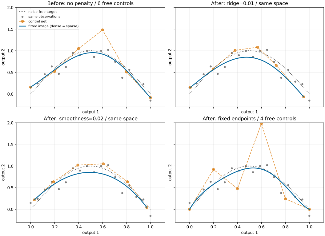
Fig. 9 The same degree-five space and 18 noisy observations before and after ridge, smoothness or endpoint constraints. Blue curves show model images; orange polygons show controls. Common axes make shrinkage and endpoint changes comparable. See Regularization and numerical evidence for the objective and weights.

This existing figure is regenerated by python examples/generate_regularization_comparison.py with plot and sparse extras. Dense/sparse prediction agreement is checked before rendering. The figure shows a real change of fitted coefficients; the resolution comparison in Grid sampling shows a change of display density only.

Residuals, boundaries and assembled domains

For observed points, compute prediction - samples.values and plot it against the relevant parameter coordinate. Inspect signed residuals to detect systematic bias and absolute or squared residuals to identify large local errors. For weighted observations, show which points have large weights; a tiny weighted MSE can coexist with large errors at nearly ignored rows. For independent test responses, use the same coordinates and units in both before/after plots.

plot_model draws maximal cells on shared axes. Shared face controls encode C0 agreement, so overlapping boundaries can be visually indistinguishable. Check explicit face predictions numerically when testing continuity. Domains above dimension two are displayed through their two-dimensional faces, not as filled high-dimensional interiors. An attractive boundary view does not establish that the interior is accurate or non-self-intersecting.

A control net illustrates coefficient locations and adjacency; it is not the surface itself. Ridge can move controls toward zero, and smoothness can bring neighbors together, without changing degree or topology. Exact subdivision changes local control nets while preserving the image. Compare actual model values on parent-mapped points when investigating a split, as shown in Exact local subdivision.

Every new guide figure can be reproduced with python examples/generate_guide_figures.py. Seeds, sample counts and measured errors are retained in the metrics JSON. The figures are synthetic illustrations of specific settings, not general accuracy or hardware performance claims. Keep numerical status and held-out errors alongside visual evidence when assessing a model for deployment.

Add a parameter-space residual view

residuals = (result.model(t) - values).detach().cpu()
fig, axes = plt.subplots(1, 2, figsize=(9, 3))
axes[0].plot(x, residuals[:, 0], "o", label="first output")
axes[0].plot(x, residuals[:, 1], "o", label="second output")
axes[0].axhline(0, color="black", linewidth=.5)
axes[0].set(xlabel="segment parameter", ylabel="signed residual")
axes[0].legend()
axes[1].plot(x, residuals.square().sum(1).sqrt(), "o")
axes[1].set(xlabel="segment parameter", ylabel="output-vector error norm")
plt.close(fig)

These are training residuals, so a small graph does not establish generalization. Repeat the calculation on independent parameter-response pairs to assess prediction. Signed residuals distinguish systematic underprediction from overprediction; the vector norm summarizes magnitude but can be dominated by an output with larger physical units.

For a product domain, plot residuals against each factor or take slices at fixed operating conditions. The simploid figure shows why one surface view cannot reveal every slice of a prism. For an assembled domain, label residuals by cell and explicitly compare paired boundary coordinates. A projected seam can look closed while an omitted output disagrees or a parameter orientation is reversed.