Single and assembled domains

Choose the domain before the degree

A Bézier simplex models a response over one simplex: a segment for two barycentric weights, a triangle for three, or a higher-dimensional trade-off domain. A simploid is a product of simplices. Use a product when independent sets of weights vary together, such as a triangular trade-off at each setting of a separate interval parameter. Use an assembled domain when several local patches must share boundaries, or when a single simplex cannot express the required topology.

These choices solve different problems. Increasing degree adds polynomial flexibility inside an existing chart. Adding a product factor introduces an independent parameter block. Gluing cells changes how charts meet. A higher degree cannot turn a segment into a loop by itself; the endpoint identification must be represented in the domain or enforced separately by the application. Likewise, choosing a square rather than a triangle changes the feasible combinations of parameters, not simply the number of learned controls.

The unified API separates four objects. SimploidalSet is a mutable topology builder. BezierSpace is an immutable compiled geometry and coefficient layout. Samples contains observations with parameter rows and cell IDs. BezierModel contains learned output coefficients in that space. fit uses those objects and always returns FitResult. No separate regression entry point is needed for products or assembled domains.

Read the square, prism and glued-patch picture

The three-panel overview gives a concrete picture of the domains used below. In its left panel, choosing one location on each of two intervals gives a square; the Bézier map bends that square into a saddle. In the middle, each triangle location can be combined with any height, giving a prism. Only its two-dimensional boundary faces are rendered. In the right panel, the triangle and square have separate charts and meet through an identified edge. Gluing does not introduce an independent parameter, whereas taking a product does.

Keep three quantities separate when reading the figure. The type gives factor dimensions, the degree gives polynomial capacity per factor, and the output count gives the ambient dimension in which the image lies. A type (1, 1) model with three outputs is a surface in three-dimensional space; a type (2, 1) model has a three-dimensional parameter domain even when the renderer shows only surfaces. Red controls describe the polynomial and are not necessarily measured points or points on the image.

Table 17 Domain choices and parameter rows

Domain	Type and dimension	Active row	Example interpretation
Triangle	(2,), dimension 2	[w0, w1, w2], sum 1	Three competing priorities
Square	(1, 1), dimension 2	[1-u, u, 1-v, v]	Two priorities and a condition
Prism	(2, 1), dimension 3	[w0, w1, w2, 1-h, h]	Three priorities and a condition
Triangle glued to square	Two maximal cells, each dimension 2	Cell ID plus its local row	Neighboring response regions

The square allows u and v both to reach one. Replacing its four columns by one sum-to-one row would change the domain, not merely its encoding. Conversely, using a prism for three coupled priority weights and a height preserves both the triangular priority constraint and independent height variation.

Single simplices and products

import torch
from torch_bsf import BezierSpace, Points, Samples, fit
from torch_bsf.sampling import sample, grid

triangle = BezierSpace.simplex(2, degree=3)
prism = BezierSpace.simploid((2, 1), degree=(3, 2))
points = sample(prism, 40, seed=7)
t = points.parameters
assert t.shape == (40, 5)
assert torch.allclose(t[:, :3].sum(1), torch.ones(40, dtype=torch.float64))
assert torch.allclose(t[:, 3:].sum(1), torch.ones(40, dtype=torch.float64))
values = (t[:, 1] + t[:, 2] * t[:, 4].square())[:, None]
result = fit(prism, Samples(points, values)).require_success()
assert prism.n_controls == 10 * 3
assert result.metrics["data_mse"] < 1e-24

The prism’s first block contains three triangle coordinates and its second contains two segment coordinates. Each block sums to one. The five-column row therefore sums to two, which is correct for a two-factor product. Normalizing the whole row to one would break both factors. Factor order is meaningful: (2, 1) and (1, 2) have the same total dimension but different column block order and degree interpretation.

A product’s dimension is the sum of factor dimensions. Its coordinate width is the sum of each dimension plus one. Its control count is the product of factor control counts. For dimensions \((a_1,\ldots,a_k)\) and degrees \((d_1,\ldots,d_k)\),

\[n_{\mathrm{controls}}=\prod_{i=1}^k\binom{a_i+d_i}{d_i}.\]

A degree-three triangle has ten controls; adding a degree-two interval gives thirty. Increasing the interval degree to four gives fifty, while leaving the triangle degree unchanged. This anisotropic capacity is useful when the response varies more strongly along one independent factor. It also increases the amount of data required to determine the coefficients reliably.

For an integer degree supplied to simploid, every factor uses that degree. For a tuple, supply one entry per factor. A zero-dimensional simplex is a constant domain with no active parameter columns. It is distinct from a degree-zero function on a nonconstant domain: the latter still has input coordinates, although its predicted value does not vary with them.

Evaluate through result.model(points). The basis is a tensor product of factor Bernstein polynomials. Outputs can have any positive column count; geometry does not depend on that count. A fitted model is a PyTorch module, so evaluation is differentiable with respect to coefficients and parameter coordinates. Numerical regression itself remains a CPU float64 solve.

Build a connected two-patch domain

Suppose a response is measured on two local intervals representing adjacent experimental regimes. Fitting them independently can give different predictions at the common endpoint, especially with measurement noise. Gluing their endpoint vertices makes the corresponding coefficients shared, so the models agree there exactly while retaining independent interior controls.

from torch_bsf.geometry import SimploidalSet
domain = SimploidalSet()
left = domain.add_simplex(1)
right = domain.add_simplex(1)
domain.identify(left.face(0, 0), right.face(0, 1))
space = BezierSpace.on_set(domain, degree=3)
u = torch.linspace(0, 1, 12, dtype=torch.float64)
local = torch.stack([1 - u, u], dim=1)
left_values = (.5 * u).square()[:, None]
right_values = (.5 + .5 * u).square()[:, None]
observations = Samples.from_cells(space, [
    (left, local, left_values),
    (right, local, right_values),
])
joined = fit(space, observations).require_success()
seam = Points.from_cells(space, [
    (left, [[0., 1.]]),
    (right, [[1., 0.]]),
])
seam_values = joined.model(seam)
assert torch.equal(seam_values[0], seam_values[1])
assert space.control_index((0, 3), cell=left) == space.control_index((3, 0), cell=right)

face(i, j) removes vertex j in factor i. On a segment, face(0, 0) leaves its second endpoint and face(0, 1) leaves its first. This indexing can initially feel reversed if you think of a face number as a vertex number. Verify endpoint coordinate rows explicitly before identifying patches. For a triangle, a face is an edge; for a product, the selected factor is reduced while all other factors remain.

The fit above uses two local charts for one global scalar response. Local coordinate u=0 on the right patch is physically different from u=0 on the left. The cell ID carries that distinction. Never concatenate local parameter arrays and discard their IDs: equal coordinates do not mean equal physical locations across charts.

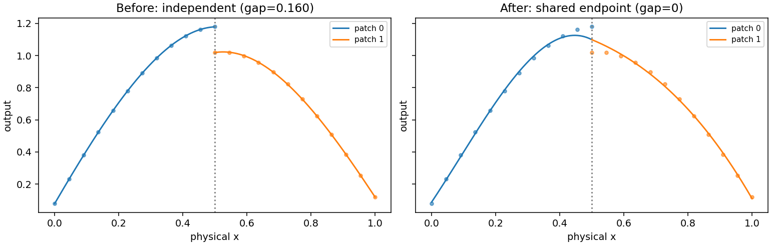
Fig. 15 Before: independent cubic patches fit offset observations and disagree at the common physical endpoint. After: one compiled space shares that endpoint coefficient. Interior residuals may increase because continuity is an exact modeling requirement. The same observations are used throughout.

Reproduce the figure with python examples/generate_guide_figures.py. The generator checks exact equality at the assembled seam and stores the before/after endpoint gap in metrics.json. This illustrates C0 continuity, not equal derivatives or a globally smooth parameterization.

Mix cell types and preserve row identity

A simploidal set can contain triangles, squares, prisms and their identified faces. For example, connect a triangle edge to a square edge:

from torch_bsf import BezierSpace, Points, Samples, fit
from torch_bsf.geometry import SimploidalSet
from torch_bsf.sampling import sample

domain = SimploidalSet()
triangle = domain.add_simplex(2)
square = domain.add_simploid((1, 1))
domain.identify(triangle.face(0, 0), square.face(0, 0))
space = BezierSpace.on_set(domain, degree=2)
triangle_points = sample(BezierSpace.simplex(2, degree=2), 30, seed=1)
square_points = sample(BezierSpace.simploid((1, 1), degree=2), 30, seed=2)
observations = Samples.from_cells(space, [
    (triangle, triangle_points.parameters, triangle_points.parameters[:, :1]),
    (square, square_points.parameters, square_points.parameters[:, :1]),
])
mixed_result = fit(space, observations).require_success()
prediction_points = Points.from_cells(space, [
    (square, square_points.parameters[:2]),
    (triangle, triangle_points.parameters[:3]),
])
assert mixed_result.model(prediction_points).shape == (5, 1)

from_cells packs rows and pads smaller charts to space.width. Only a row’s active cell coordinates are evaluated. The returned prediction order matches the supplied batch order, so the first two predictions above belong to the square and the next three to the triangle. For observations, retain that same order for values and weights.

Points(parameters, cell_ids) offers direct construction when you already have padded arrays. Use integer cell IDs with one ID per row. The immutable space validates that coordinates belong to each cell’s simplex factors. Multi-cell models require explicit Points even if every cell has the same width; untagged tensors cannot choose between two charts safely.

space.n_cells includes addressable lower-dimensional faces as well as maximal patches. space.main_cells identifies maximal cells used by default sampling and plotting. Do not assume those IDs are consecutive top-level patch numbers or equal to builder insertion order. Resolve builder handles with space.cell_id(handle) and preserve the resolved IDs in exported observation files.

Degree propagation across shared faces

Identified faces have one polynomial representation, so their degrees must be compatible. BezierSpace.on_set(domain, degree=2) applies a common degree to every factor. A mapping can specify selected cell/factor degrees; the compiler propagates them through shared faces. Use default_degree for factors still undetermined after propagation. Inconsistent assignments raise rather than quietly elevating degrees or weakening continuity.

For example, a prism’s triangle-face degree must match an attached triangle’s degree. Its independent interval degree can differ if no shared relation constrains it. This is why “one degree per cell” is not always an independent choice. Degrees belong to factors, and connected face relationships can tie together assignments that look separate in a drawing.

Increasing a degree adds controls and permits more variation, while also increasing fitting work and potentially worsening identifiability. It does not repair an incorrect face identification or inconsistent chart orientation. Check geometry with simple endpoint and face examples before fitting noisy high-dimensional data. For assembled spaces, degrees must be at least one; use a standalone constant space for constant-domain regression.

To inspect a local coefficient, use space.control_index(index, cell=handle). For a product, index contains one multi-index per factor. Two references on an identified face may resolve to the same global row. The global coefficient matrix stores that row once, so optimizing or fixing it changes all incident cells consistently. Do not edit several apparent copies and expect independent effects; there is only one shared unknown.

The immutable space snapshots the builder. Adding or identifying more cells later does not alter an existing model’s geometry. Compile a new space and fit or explicitly transfer values when the topology changes. This separation makes archived models independent of later mutations to experiment setup. It also means builder edits alone cannot update a previously created model.

Continuity and exact constraints

Shared coefficients enforce C0 continuity: cell predictions agree on the identified face. They do not automatically enforce tangent agreement, C1 continuity, injectivity, manifold orientation or lack of self-intersections. A visually smooth projection is insufficient evidence for any of those properties. Evaluate the particular derivative or geometric condition your application requires.

If an entire boundary response is known, fixing its complete control net prescribes that polynomial exactly. Fixing only boundary vertices prescribes only vertex values at higher degree. FixedControls.from_cells resolves local references into shared global rows and rejects conflicting values. When observations on opposite sides of a seam disagree, the fitted shared boundary compromises according to their relative weights unless it is fixed.

Smoothness penalizes adjacent coefficient differences in the global net. It can reduce variation, but it is not a derivative-matching condition between charts. Its effect depends on degree and adjacency as well as its weight. Keep geometry, exact constraints and soft regularization conceptually separate when interpreting a before/after comparison. See Regularization and numerical evidence and Fixed controls for their objectives and tuning guidance.

Sampling and visual checks

sample(space, n, seed=...) chooses maximal cells with equal probability by default, then samples uniformly in their factor charts. This is not uniform physical area on a curved fitted surface. Supply cell weights when your experiment budget should favor some patches. If every patch needs observations, allocate them explicitly instead of relying on expected counts.

grid visits every selected maximal chart and includes its boundary lattice. Shared physical boundary points can appear as several chart-tagged rows. Keep both when checking C0 agreement, but account for duplication when calculating a physical integration rule or pooled region metric. A low-dimensional face with few observations can still be underdetermined even if the whole assembled data set is large.

plot_model draws all maximal cell images on common axes. It displays higher-dimensional domains through two-dimensional faces. For mixed patches, overlay observations with distinct markers and inspect residuals per cell. A global average error can hide failure on a small but important patch. Projecting to two outputs can also hide disagreement in another output.

For an exact local subdivision, retain subdivide parameter maps and compare children in parent coordinates. That operation does not automatically remesh adjacent assembled patches. Rebuild the domain explicitly if the refined pieces must share new boundaries with their neighbors. See Exact local subdivision for the distinction between exact reparameterization and additional local fitting.

Persistence and troubleshooting

save_model preserves compiled cells, stable IDs, shared layout and learned coefficients. A restored model does not need the mutable builder or its original Python handles. For new observations after loading, use saved integer IDs and the recorded chart conventions. A CSV of control coordinates alone cannot reconstruct topology or shared coefficient relationships.

If a prediction rejects a row, first check its cell ID, active width and per-factor sums. If two supposed boundary points disagree, check that they are actually paired by the declared identification and that their local coordinates have matching orientation. If fitting succeeds but coefficients are unidentifiable, inspect per-cell observation coverage and data diagnostics; regularizing the assembled system does not add missing measurements.

When choosing between one high-degree chart and several glued low-degree charts, compare held-out error, total controls, boundary requirements and maintenance of coordinate maps. Several patches can capture local structure, but they require explicit chart identity and topology. Prefer the simplest domain that matches the experiment’s feasible parameter combinations and required global connectivity, then tune its degree with validation.

Homology

The topology of a simploidal set can be checked after it is built by computing its homology (Section 4.4 of Peltier and Lienhardt [PL18]). The chain group \(C_k\) is spanned by the non-degenerate simploids of dimension \(k\), and the boundary of a simploid \(\sigma\) of type \((a_1, \ldots, a_n)\) follows the sign rule of a product of simplices:

\[\partial \sigma = \sum_{i=1}^n \sum_{j=0}^{a_i} (-1)^{a_1 + \cdots + a_{i-1} + j} d^i_j \sigma,\]

where the terms whose face \(d^i_j \sigma\) is degenerate are dropped.

• boundary_matrix() returns the integer matrix of \(\partial_k\), with rows simploids(k - 1) and columns simploids(k); it satisfies boundary_matrix(k) @ boundary_matrix(k + 1) == 0.

• betti_numbers() returns the Betti numbers \(\beta_0, \ldots, \beta_{\dim}\), the ranks of the homology groups. The ranks are computed exactly by integer elimination, over the rationals (field="Q", default) or over \(\mathbb Z / 2\) (field="Z2"); the two differ only for spaces whose integral homology has torsion, such as non-orientable surfaces.

from torch_bsf.geometry import SimploidalSet

# A torus: a square whose opposite edges are identified
torus = SimploidalSet()
square = torus.add_simploid((1, 1))
torus.identify(square.face(0, 0), square.face(0, 1))
torus.identify(square.face(1, 0), square.face(1, 1))
print(torus.betti_numbers())

# A sphere: a square whose two edges face(1, *) are collapsed into
# vertices and whose two other edges are identified
sphere = SimploidalSet()
square = sphere.add_simploid((1, 1))
for j in range(2):
    edge = square.face(1, j)
    sphere.degenerate(edge, edge.face(0, 0), 0, -1)
sphere.identify(square.face(0, 0), square.face(0, 1))
print(sphere.betti_numbers())

# A projective plane: two triangles glued along their edges
rp2 = SimploidalSet()
t1, t2 = rp2.add_simplex(2), rp2.add_simplex(2)
rp2.identify(t1.face(0, 0), t2.face(0, 0))
rp2.identify(t1.face(0, 1), t2.face(0, 2))
rp2.identify(t1.face(0, 2), t2.face(0, 1))
print(rp2.betti_numbers(), rp2.betti_numbers(field="Z2"))

[1, 2, 1]
[1, 0, 1]
[1, 0, 0] [1, 1, 1]

Topological checks complement numerical checks

Betti numbers describe connectivity and holes of the declared domain, not properties inferred from observations. A torus domain remains topologically a torus even if learned coefficients collapse its image to a point. Conversely, a self-intersecting plotted image does not automatically change the builder’s homology. Inspect the domain and its fitted image separately.

Use domain.check() before compilation, examine expected component and hole counts, and then verify representative identified-face predictions numerically. If a collapsed edge is represented through degeneracy, confirm that the fitted image is constant along that direction. These small checks often reveal chart mistakes earlier than a large regression or expensive experiment batch. For the categorical background and face/degeneracy relations, see The Category of Simploidal Sets.

Plan an assembled experiment from end to end

Begin with a small geometric sketch that names every local chart and its parameter convention. List which faces represent the same physical boundary and whether their parameter direction agrees. Then construct only those identifications and verify them using simple coefficient values or a known response. This is easier to diagnose than fitting a large noisy data set and trying to infer a mistaken orientation from the resulting image.

Allocate observations per maximal patch and deliberately include important shared boundaries. Boundary measurements can be entered through their face cell or through either incident chart, provided the chosen coordinates and IDs are consistent. If the same physical measurement is entered twice, it receives twice the relative influence unless weights account for duplication. Decide whether two rows are independent experiments or two chart descriptions of one experiment before forming the final Samples object.

Check control counts after compilation rather than summing standalone patch counts: sharing reduces the number of independent unknowns. Conversely, a large total observation count does not imply that every patch is sufficiently sampled. Build a per-cell summary of row count, total weight and held-out residuals. This often identifies a poorly covered patch before global data rank or a global error statistic makes the underlying cause obvious.

When comparing topology choices, keep the measured responses and physical evaluation locations fixed. An independently fitted pair of patches has more free boundary values than a glued pair, so its training residual may be lower. That does not make it preferable when continuity is a requirement. Report both held-out accuracy and the boundary agreement condition, as the seam figure does. For higher-dimensional faces, compare a grid over the whole face, not just its corners.

After the geometry and validation protocol are stable, increase degree or add penalties one change at a time. Recompile when topology changes, resolve fixed rows again, and preserve the mapping from raw-data chart names to stable saved IDs. That mapping makes model archives useful to future experiments without depending on the lifetime of the original topology builder.

Retain that validated domain schema alongside every exported observation batch.

High-degree evaluation

Bernstein factors of degree 16 and above use degree elevation rather than forming a large multinomial times a tiny monomial. This keeps finite nonnegative barycentric inputs on their simplex finite at degrees such as 20 (float16), 140 (float32), and 171 (float64), including vertices and faces. The polynomial recurrence preserves coordinate and coefficient autograd at zero coordinates. Rounding error grows with degree and factor count; very small basis entries can still underflow in the requested dtype.

The recurrence retains intermediate bases for autograd and performs work proportional to the sum of control counts over all lower degrees. Large control counts are still limited by available memory. Predecessor index tables are cached per degree, factor width and device for the lifetime of the process to avoid rebuilding and transferring them on repeated evaluations. Extrapolation outside the simplex can overflow when the polynomial itself is not representable. Gram integration combines moments and multinomials in the log domain. Its explicit multinomials must fit float64, otherwise it raises ValueError explaining that degree limit. Point-cloud fitting uses the same recurrence for high-degree values and first/second derivatives; its optimization and least-squares conditioning limits still apply.