Output scaling
When and why to change output coordinates
A surrogate may predict quantities with very different units, such as latency in seconds and energy in joules. Their numerical ranges can differ by several orders of magnitude. Plotting raw outputs can hide the smaller response, and an error metric that averages squared output errors can be dominated by the larger one. Explicit scaling makes the choice of relative units visible and can make comparisons and optimization gradients easier to interpret.
Core regression does not normalize automatically. fit defines residuals,
ridge and smoothness in the output coordinates you provide. This is intentional:
normalizing a response changes the meaning of zero, and therefore can change
the prior expressed by a penalty. Choose units according to the prediction
problem, retain the transformation, and invert it before reporting physical
errors or sending predictions to downstream software.
Output scaling is separate from parameter coordinates. A simplex input row must still contain nonnegative barycentric values summing to one. Never apply an ordinary feature standardizer independently to those columns and then pass them to a Bézier space: the resulting rows will generally leave the domain. For a product domain, each barycentric factor has its own sum-to-one constraint.
A complete explicit transformation
This example standardizes two responses, fits the transformed observations, and restores predictions. Every tensor is float64 so that comparisons probe the transformation rather than float32 rounding of large offsets.
import torch
from torch_bsf import BezierSpace, Samples, fit
from torch_bsf.preprocessing import StdScaler

x = torch.linspace(0, 1, 21, dtype=torch.float64)
t = torch.stack([1 - x, x], dim=1)
values = torch.stack([x.square(), 1000 + 100 * x.square()], dim=1)
space = BezierSpace.simplex(1, degree=2)
scaler = StdScaler()
transformed = scaler.fit_transform(values)
scaled_result = fit(space, Samples(t, transformed)).require_success()
restored = scaler.inverse_transform(scaled_result.model(t))
direct_result = fit(space, Samples(t, values)).require_success()
assert torch.allclose(restored, direct_result.model(t), atol=1e-10)
The scaler’s statistics are fitted once to training outputs. Apply
transform to later observations with those same statistics; do not refit
them at prediction time. inverse_transform expects the same output-column
order. If column names or units change, update the transformation and model
together rather than silently reusing old statistics.
The model archive stores the learned model in its current coordinates. It
does not package an arbitrary preprocessing object. Save the scaler’s numeric
statistics and column schema through your application, and apply the inverse
transformation when loading the model. A .bsf extension does not imply that
normalization has been inferred or remembered.
Choose a scaler
Scaler |
Transform |
When to try it |
|---|---|---|
|
Subtract column minimum and divide by its training range. |
Known bounded responses; a convenient nominal zero-to-one scale. |
|
Subtract column mean and divide by its training standard deviation. |
Compare variations relative to typical observed spread. |
|
Use lower and upper quantiles as the reference range, without clipping. |
Extreme observations would dominate a min-max scale. |
|
Identity transform and inverse. |
Keep original units within a common preprocessing workflow. |
Min-max scaling maps the training extrema to zero and one, but future observations may fall outside that interval. Standardization does not bound values at all. Quantile scaling is an affine change of units based on robust reference points, not a nonlinear transform to a uniform distribution. Values outside the selected quantile interval remain below zero or above one; they are not clipped or discarded.
QuantileScaler exposes its lower quantile fraction as q (default .05).
Set it before fitting, for example scaler = QuantileScaler(); scaler.q = .1.
Use 0 <= q < .5 so the reference interval is ordered and has a meaningful
width. Increasing q ignores more tail observations when defining the
reference range, usually reducing the divisor and making tails numerically
larger after transformation. It does not reduce their regression weights.
If robust fitting rather than robust scale estimation is required, this
transform alone does not implement it.
Constant output columns use a divisor of one to avoid division by zero.
StdScaler also guards its single-sample standard deviation. Near-constant
columns can still have tiny nonzero ranges: check fitted statistics and decide
whether amplifying their noise is useful. The supplied scalers estimate
unweighted column statistics. Observation weights supplied to Samples do
not automatically change those statistics; calculate an application-specific
weighted transform when that is the intended meaning.
What changes mathematically?
For one output, write the transform as \(z=(y-a)/s\), with nonzero scale \(s\). Bernstein bases contain constants, so transforming each control \(Q=(P-a)/s\) gives the corresponding transformed polynomial. Without penalties or constraints, affine scaling leaves the exact least-squares predictions unchanged after inversion. It can change numerical rounding, but is not a mechanism for making an unregularized independent-column fit more expressive or statistically more accurate.
This observation also applies to multiple independent outputs: rescaling an output multiplies its data objective by a positive constant, without coupling it to other output columns. However, reported aggregate errors and acquisition scores do change their relative weighting across columns. Distinguish the model solution from the statistic used to rank competing models or queries.
With ridge, centering changes the preferred origin. Penalizing \(\|Q\|^2\) favors output \(a\) after inversion, whereas penalizing \(\|P\|^2\) favors original zero. Smoothness uses differences between neighboring controls and is invariant under translation. Pure multiplicative scaling of an independent output scales its data and quadratic penalty terms together, so it need not change its inverse-transformed optimum at unchanged penalty weights. Avoid assuming that every change of units automatically requires a different fitted curve. Check the exact transform, objective and cross-output selection criterion.
Fixed values must be transformed by the same affine rule as observations.
If a known endpoint is 1000 in original units, fixing it to 1000 inside a
standardized fit imposes an entirely different constraint. Transform its
one-row output tensor, then create FixedControls from that transformed
value. Invert predictions before checking agreement with physical boundary
conditions. See Fixed controls for resolving coefficient indices.
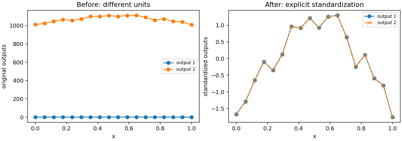
Fig. 7 Before: the larger output offset hides the smaller response. After: explicit standardization makes both variations visible. This display change does not claim improved unregularized fitting accuracy: the generator verifies that inverse-transformed and direct predictions agree.
The comparison uses a cubic model and the same noisy observations in both
outputs, with the second output translated and scaled. Reproduce it with
python examples/generate_guide_figures.py; the maximum inverse-prediction
difference is recorded in metrics.json.
Validation without leakage
Fit preprocessing on each training fold, transform that fold’s held-out
outputs with the training statistics, predict, invert, and evaluate in the
units that matter. Fitting the scaler on all outputs before splitting uses
test information. For a regularized fit, that can also change its preferred
origin using held-out data. The convenience cross_validate function does
not fit preprocessing objects for you.
A practical manual fold loop uses KFold.split(len(samples)) and
samples.take(indices). Create a fresh scaler in each iteration. Keep
original held-out values for reporting error, and use the same fold partitions
for every degree and penalty comparison. If you select candidates by
standardized error, explain that each output is weighted relative to its
training spread; if you select by original-unit error, report the units and
output-specific tolerances.
After selection, refit the scaler on all available training data and train a fresh model with the chosen settings. Keep a final untouched test set if one is needed. See Cross-validation and degree search for metrics and Explicit ensembles and active learning for how changing output scales changes committee disagreement rankings.
Extreme finite values
The scalers require nonempty finite input tables. StdScaler and
QuantileScaler require floating values; MinMaxScaler also accepts
integral tensors. For floating input, statistics and transformed outputs must
fit the input dtype. Standard deviations and quantiles retry with scaled
arithmetic when ordinary reductions overflow; constant and single-sample columns retain their
unit-scale convention. Transforms and inverse transforms also retry a factored
affine expression when a subtraction or product overflows before cancellation.
The fitted public scales / stds attributes remain single tensors in the
original units. If a range or sample standard deviation itself exceeds that
dtype, fitting raises ValueError with a recommendation to rescale the
original units. For example, float64 [-1e308, 1e308] has an unrepresentable
min-max range (2e308), although its sample standard deviation is representable.
The min-max and default quantile scalers reject this range explicitly; the
standard scaler returns approximately [-0.7071, 0.7071]. Divide the original
data by a suitable unit (for example 1e308) before fitting when needed,
and retain that unit separately for interpreting inverse transforms.
Non-finite input and genuinely unrepresentable forward or inverse results also
raise ValueError instead of propagating NaN/Inf. A successful inverse is
still subject to floating rounding: a spread smaller than the precision of a
large offset may already have been lost in the supplied data. These scalers do
not recover information absent from the input dtype. NoneScaler remains a
pass-through, without numerical validation.
A varying column whose nonzero standard deviation rounds to zero also raises
ValueError. The unit-scale convention applies to genuinely constant
columns and single samples. Scale tiny original units upward before fitting;
otherwise substituting a unit standard deviation would silently skip
standardization of varying data.
For integral MinMaxScaler input, fitted minima and ranges retain their
integer dtype; a range exceeding that dtype raises ValueError before
subtraction can wrap. Subtraction happens before true division, preserving adjacent
integer differences even at large offsets. Normalized values follow PyTorch’s
default floating dtype; half outputs use float32 division before casting to
that dtype. A remaining nonfinite integer transform uses exact rational CPU
arithmetic before rounding once to the output dtype; this preserves the last
finite half rounding interval. Floating inverse results have floating precision, so adjacent
large integers can round together in that output dtype. Boolean and complex
inputs remain unsupported. Integer extrapolation retries a floating expression
when subtraction would wrap. Integer inputs to inverse_transform keep their
promoted integer output dtype: risky multiplication or addition uses exact
Python integers on the CPU, and a final result outside that dtype raises
ValueError. Ordinary integer inverse operations stay on the tensor device.