Data Normalization

Proper normalization of your data is crucial for stable and accurate Bézier simplex fitting, as both the input parameters and the output values should ideally be within a well-defined range.

Parameter Normalization

The fit() function expects each row of the params tensor to lie on the standard simplex \(\Delta^{M-1}\) (i.e., the elements must be non-negative and sum to 1). If your raw parameters do not satisfy this condition, you must normalize them manually before fitting.

A common approach is L1 Normalization: divide each parameter vector by its \(\ell_1\) norm. For parameters \(a, b \ge 0\), you can compute the simplex coordinates as \(t_1 = a / (a + b)\) and \(t_2 = b / (a + b)\).

# Manual L1 normalization for parameter tensors
ts = ts / ts.sum(dim=1, keepdim=True)

While the best normalization method depends on your specific problem, the L1 approach is a solid default. If your parameter space does not naturally have a simplex structure and no intuitive normalization seems appropriate, it is possible that the problem is not well-suited for Bézier simplex fitting.

Value Normalization

Normalizing the output values (the targets) can help the optimizer converge faster by ensuring that different objectives are on a similar scale. In the CLI or MLflow interface, you can use the --normalize argument.

Available options include:

max: Scales values to the range [0, 1] based on the observed maximum. This is suitable when the training data covers the full expected range (upper and lower bounds) for all axes.
std: Standardizes values to have zero mean and unit variance. This is the most common choice for general datasets.
quantile: Transforms values based on quantiles. This is robust to outliers and is recommended when the training data contains significant extremes that might otherwise skew the scaling.

from torch_bsf.preprocessing import StdScaler

# Normalize values using the internal StdScaler
scaler = StdScaler()
xs_normalized = scaler.fit_transform(xs)

# Fit the model (remember to use normalized values)
bs = torch_bsf.fit(params=ts, values=xs_normalized, degree=3)

# To predict and get results in the original scale
t_new = [[0.2, 0.3, 0.5]]
x_normalized = bs(t_new)
x_original = scaler.inverse_transform(x_normalized)

While normalization can often improve prediction accuracy and training stability, it is not a guarantee. You should select the method that best aligns with your data distribution to achieve the best results.

Advanced Considerations

Numerical stability and fitting accuracy also depend on how your data points are distributed within their ranges.

Parameter Space Uniformization

Bézier simplex fitting performs most effectively when the training data is uniformly distributed across the entire simplex. If your samples are clustered in certain regions (skewed), the model may struggle to accurately represent the surface in sparse areas, even if the total number of samples is large.

If your data is naturally biased, consider applying a transformation to “uniformize” the distribution before fitting. For example, when exploring hyperparameters such as those generated by torch_bsf.model_selection.elastic_net_grid (which often uses log-spaced \(\lambda\)), the data is heavily concentrated at one end of the simplex. In such cases, fitting on the “raw” biased parameters can lead to significantly higher errors than fitting on uniform data.

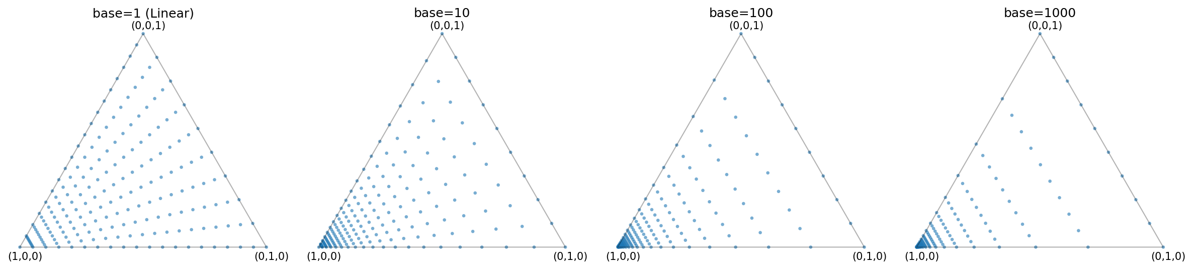
Comparison of elastic_net_grid with different base values. — Fig. 5 Distribution of points generated by `elastic_net_grid` for different `base` values. As the `base` increases, the points are more heavily concentrated towards a corner of the simplex.

In practice, when using such skewed grids, it is often more effective to perform the Bézier simplex fitting using the grid indices (which are uniformly spaced) and then map the results back to the original parameter space.

Table 1 Impact of Parameter Distribution (3rd Degree Simplex)
Parameter Sampling Strategy	Test MSE
Uniform Triangular Grid	1.92e-04
Skewed (Log-grid style, base 1000)	4.28e-03

Preserving Physical Scales in Values

The objective function in PyTorch-BSF (Mean Squared Error) is calculated in the normalized value space whenever normalization is applied.

Automatic Balancing: Scaling all axes to [0, 1] ensures that each objective contributes roughly equally to the training process, regardless of its original unit or magnitude.
Physical Significance: However, if the absolute magnitude of an axis has physical meaning or represents its relative importance, you may choose not to scale. For instance, if one objective ranges from 0 to 1 and another from 0 to 1000, and you want the optimizer to prioritize absolute precision on the larger objective, leaving the data unscaled will naturally cause the larger values to dominate the loss function.

Carefully consider whether you want all objectives to be weighted “fairly” according to their variance, or weighted “physically” according to their raw magnitudes.