Pareto Set Learning by Stochastic Gradient Descent

torch_bsf.fit() fits a model to data: Pareto-optimal solutions computed beforehand. When the objective functions themselves are available, torch_bsf.fit_sgd() fits the model to the Pareto set directly, with the preconditioned stochastic gradient descent of Hikima et al. [HKT+25]. It works with every model of torch_bsf.simploidal: Bézier simplices, Bézier simploids and simploidal Bézier spaces (see Simploidal Sets).

The algorithm

Let \(f = (f_1, \ldots, f_M): \mathbb R^L \to \mathbb R^M\) be the objectives and \(b(\mathbf t \mid P) = P^\top \mathbf z(\mathbf t)\) a Bézier simplex of degree \(D\) on \(\Delta^{M-1}\), where \(\mathbf z(\mathbf t)\) is the vector of the Bernstein basis polynomials. The paper minimizes the linear scalarization weighted by the parameter itself, averaged over the simplex:

\[\mathcal L(P) = \mathbb E_{\mathbf t \sim U(\Delta^{M-1})}\bigl[\mathbf t^\top f(b(\mathbf t \mid P))\bigr].\]

For strongly convex objectives, the minimizer of \(\mathbf t^\top f(\mathbf x)\) traces the whole Pareto set as \(\mathbf t\) moves on the simplex, so the minimizer of \(\mathcal L\) approximates the Pareto set, parametrized by the weight.

The expectation is replaced by the mean over \(n\) fixed samples \(\mathbf t_1, \ldots, \mathbf t_n\), and the control points are updated on minibatches \(B\) of them:

\[P^{(k+1)} = P^{(k)} - \alpha_k \Sigma^{-1} \nabla \mathcal L_B(P^{(k)}), \qquad \Sigma = \mathbb E_{\mathbf t \sim U(\Delta^{M-1})}\bigl[\mathbf z(\mathbf t)\,\mathbf z(\mathbf t)^\top\bigr].\]

The preconditioner \(\Sigma^{-1}\) turns the step into the one that minimizes the linearized loss plus \(\frac{1}{2\alpha_k}\mathbb E_{\mathbf t}\|b(\mathbf t \mid P) - b(\mathbf t \mid P^{(k)})\|^2\): it measures how far the surface moves rather than how far its control points move. The paper proves that this converges faster than plain SGD (\(\Sigma = I\)), whose steps are distorted by the ill-conditioning of the Bernstein basis. gram_matrix() computes \(\Sigma\) exactly, and it is factorized once.

Fitting a Bézier simplex to a Pareto set

The objectives \(f_m(\mathbf x) = \|\mathbf x - \mathbf e_m\|^2\) (\(m = 1, 2, 3\)) have the triangle spanned by \(\mathbf e_1, \mathbf e_2, \mathbf e_3\) as their Pareto set, reached at \(\mathbf x = \mathbf t\). Write the objectives for a batch of points, wrap them with linear_scalarization(), and pass an initial model, which fixes the type, the degree and the dimension \(L\):

import torch
import torch_bsf
from torch_bsf.simploidal import BezierSimploid, linear_scalarization, sample_domain

def objective(x):  # (batch, L) -> (batch, M)
    return ((x.unsqueeze(1) - torch.eye(3)) ** 2).sum(dim=-1)

init = BezierSimploid.zeros((2,), 2, n_values=3)  # a quadratic Bézier triangle in R^3
loss = linear_scalarization(objective)
bs = torch_bsf.fit_sgd(init, loss, n_samples=100, batch_size=20, max_iter=100, step_size=0.2, seed=0)

(t,) = sample_domain(bs, 1000, seed=1)  # fresh samples to check generalization
print(torch.allclose(bs(t), t, atol=1e-3))

True

The main options are:

• batch_size and n_samples: the minibatch size \(m\) and the number \(n\) of fixed samples (or pass your own samples as inputs);

• step_size and step_decay: a constant step \(\alpha\), or \(\alpha / \sqrt{k + 1}\) with step_decay="sqrt";

• preconditioner="none": plain SGD, the baseline of the paper.

The paper uses \(P_0 = O\), \(n = 100\), \(m = 20\), 100 iterations and \(\alpha = 0.05\), which are the defaults except for the minibatch size (full batch by default). The returned model is a copy, so init can be reused.

Monitoring the loss and stopping early

Pass callback to watch the fitting. After the update of every iteration \(k = 0, 1, \ldots\), fit_sgd() calls callback(k, model, batch_loss), where model is the model being fitted (already updated) and batch_loss is the mean loss of the minibatch at the parameters before the update, i.e., \(\mathcal L_B(P^{(k)})\). To compare the empirical loss on the fixed samples with the generalization loss on fresh ones, as the paper does, pass the samples as inputs and evaluate the model on both in the callback, under torch.no_grad():

inputs = sample_domain(init, 100, seed=0)  # the samples fit_sgd minimizes on
test_inputs = sample_domain(init, 1000, seed=1)  # fresh samples

def mean_loss(model, inputs):
    with torch.no_grad():
        return loss(model(*inputs), *inputs).mean().item()

history = {"minibatch": [], "empirical": [], "generalization": []}

def record(k, model, batch_loss):
    history["minibatch"].append(batch_loss)  # at P^(k)
    history["empirical"].append(mean_loss(model, inputs))  # at P^(k+1)
    history["generalization"].append(mean_loss(model, test_inputs))  # at P^(k+1)

bs = torch_bsf.fit_sgd(init, loss, inputs=inputs, batch_size=20, step_size=0.2, seed=0, callback=record)
print(len(history["empirical"]))
print(history["generalization"][-1] < history["generalization"][0])

100
True

and plot the records, e.g., with matplotlib:

import matplotlib.pyplot as plt

for name, values in history.items():
    plt.plot(values, label=name)
plt.xlabel("iteration")
plt.ylabel("loss")
plt.legend()
plt.show()

If the callback returns True, the fitting stops after that iteration and returns the model updated so far. There is no built-in stopping criterion; write one in the callback. For example, stop once the empirical loss decreases by less than \(10^{-6}\) in an iteration:

losses = []

def converged(k, model, batch_loss):
    losses.append(mean_loss(model, inputs))
    return k > 0 and losses[-2] - losses[-1] < 1e-6

bs = torch_bsf.fit_sgd(init, loss, inputs=inputs, max_iter=1000, step_size=0.2, seed=0, callback=converged)
print(len(losses) < 1000)

True

The callback receives the model being fitted, not a copy: it may evaluate the model but must not modify it. To keep a snapshot, e.g., of the best model so far, copy its parameters (model.control_points.detach().clone() for a Bézier simploid, model.proper_control_points.detach().clone() for a simploidal Bézier space). The callback does not change the fitting: a callback that never returns True gives the same model as no callback.

Freezing control points and smoothing

The minimizer of each single objective \(f_m\) is often known in advance. It is the vertex \(\mathbf t = \mathbf e_m\) of the Pareto set, so you can put it in the initial model and keep it there with freeze, as in torch_bsf.fit(). smoothness_weight adds the smoothness penalty \(w \sum_{(p, q)} \|P_p - P_q\|^2\) over the adjacent control points to the loss, which keeps the control net of a high degree model from oscillating:

init = BezierSimploid.zeros((2,), 3, n_values=3)  # a cubic Bézier triangle
vertices = [(3, 0, 0), (0, 3, 0), (0, 0, 3)]
with torch.no_grad():
    for m, vertex in enumerate(vertices):
        init[vertex].copy_(torch.eye(3)[m])  # the minimizer of f_m

bs = torch_bsf.fit_sgd(
    init, loss, freeze=vertices, smoothness_weight=1e-4, batch_size=20, max_iter=200, step_size=0.2, seed=0
)
print(all(torch.equal(bs[v], init[v]) for v in vertices))
print(torch.allclose(bs(t), t, atol=1e-2))

True
True

The frozen control points keep their values in init bit for bit. For a Bézier simplex, give their multi-indices (or full indices, as ((3, 0, 0),)); for a Bézier simploid, their indices; and for a simploidal Bézier space, pairs (simploid, index) of any simploid of the set and an index of its control net, as in fit_simploidal_set().

With frozen rows, the step moves only the free rows \(F\) and is preconditioned by the block \(\Sigma_{FF}\) of the Gram matrix rather than by \(\Sigma\), so that it still minimizes the linearized loss plus the move of the surface while the frozen rows stay fixed:

\[P_F^{(k+1)} = P_F^{(k)} - \alpha_k (\Sigma_{FF} + 2 \alpha_k w L_{FF})^{-1} \nabla_F \bigl(\mathcal L_B(P^{(k)}) + w \operatorname{tr}(P^{(k)\top} L P^{(k)})\bigr),\]

where \(L\) is the Laplacian of the adjacency graph of the control points, so that the penalty is \(w \operatorname{tr}(P^\top L P)\). The term \(2 \alpha_k w L_{FF}\) comes from minimizing the penalty exactly instead of following its gradient. The surface metric \(\Sigma\) is tiny along oscillating control nets, so \(\Sigma^{-1} L\) has eigenvalues in the thousands already for a cubic Bézier triangle, and a plain gradient step on the penalty would diverge unless \(\alpha w\) were tiny; the exact treatment is stable for every \(w\). The matrix is factorized once (once per iteration with step_decay="sqrt" and \(w > 0\)). Without frozen rows and with \(w = 0\), the step is the one of the paper.

Generalization to simploids and simploidal spaces

Every model of torch_bsf.simploidal is linear in its control points, model(*inputs) == model.design_matrix(*inputs) @ P, so the algorithm applies to all of them with \(\mathbf z(\mathbf u)\) the row of the design matrix and \(\mathbf u\) uniform on the domain of the model:

• For a Bézier simploid of type \((a_1, \ldots, a_n)\), \(\mathbf u\) is uniform on the product of simplices, and \(\Sigma\) is the Kronecker product of the Gram matrices of its factors.

• For a simploidal Bézier space, \(\mathbf u\) lies on the simploid \(c\) with probability \(w_c\) and is uniform on it, so \(\Sigma = \sum_c w_c S_c^\top \Sigma_c S_c\), where \(S_c\) maps the stored control points to the control net of \(c\). By default the weights are uniform over the main simploids (those that are not a face of another); pass weights to change them. They must cover every stored control point, so that \(\Sigma\) is invertible.

The loss is any function loss(values, *inputs) returning one value per sample, where values is the output of the model and inputs are its arguments: (t,) for a Bézier simploid and (t, simploid_ids) for a space (see sample_domain()). linear_scalarization() needs one parameter per objective, i.e., a Bézier simplex; on other domains, choose how the parameters weight the objectives. For example, on a square \((u_0, u_1) \times (v_0, v_1)\), the weights \((u_0 v_0, u_0 v_1, u_1 v_0, u_1 v_1)\) of four objectives sweep the tetrahedron of weights along a bilinear patch:

from torch_bsf.simploidal import gram_matrix

def objective4(x):
    return ((x.unsqueeze(1) - torch.eye(4)) ** 2).sum(dim=-1)

def loss4(x, t):
    w = (t[:, :2].unsqueeze(2) * t[:, 2:].unsqueeze(1)).flatten(1)  # (batch, 4)
    return (w * objective4(x)).sum(dim=-1)

init = BezierSimploid.zeros((1, 1), 1, n_values=4)
patch = torch_bsf.fit_sgd(init, loss4, batch_size=20, step_size=0.2, seed=0)
print(torch.allclose(patch.control_points, torch.eye(4), atol=1e-3))
print(gram_matrix(init).shape)

True
torch.Size([4, 4])

A simploidal Bézier space is fitted in the same way; the loss then also receives the index of the simploid of every sample.

From the command line and MLflow

python -m torch_bsf sgd fits a Bézier simplex to the Pareto set of objectives written in Python, without writing a script. Put the objectives in a module that can be imported from the current directory (or from an installed package), e.g. problems.py:

import torch

def objective(x):  # (batch, L) -> (batch, M), differentiable with PyTorch
    return ((x.unsqueeze(1) - torch.eye(3)) ** 2).sum(dim=-1)

and pass it as --objective=MODULE:FUNCTION with the number \(M\) of objectives, the number \(L\) of variables and the degree:

python -m torch_bsf sgd \
  --objective=problems:objective \
  --n-objectives=3 --n-variables=3 --degree=2 \
  --n-samples=100 --batch-size=20 --max-iter=100 --step-size=0.2 \
  --step-decay=constant --preconditioner=gram --seed=0 \
  --meshgrid=meshgrid.csv

It starts from \(P_0 = O\) and minimizes the linear scalarization on a Bézier simplex on \(\Delta^{M-1}\), as the first example above. The options --n-samples, --batch-size, --max-iter, --step-size, --step-decay, --preconditioner and --seed are those of torch_bsf.fit_sgd(), with the same defaults (each one is also accepted with underscores, e.g. --batch_size). The outputs follow the data fitting command python -m torch_bsf:

• the control points are saved to <module>.<function>,control_points,t_<M-1>,d_<N>.csv, or to the file given by --save in the format chosen by its extension;

• if --meshgrid is a CSV file of parameters (\(M\) columns), the fitted model is evaluated on them and saved to <module>.<function>,meshgrid,t_<M-1>,d_<N>.csv; nothing is evaluated if it is omitted or a directory;

• unless --loglevel=0, the options and the final loss train_loss (the mean loss over the samples) are logged to MLflow, together with the control points file and the model with --loglevel=2 (the default), and so is the loss batch_loss of the minibatch of every iteration, as a metric whose step is the iteration k.

The options of Freezing control points and smoothing and Monitoring the loss and stopping early are also available:

python -m torch_bsf sgd \
  --objective=problems:objective \
  --n-objectives=3 --n-variables=3 --degree=3 \
  --init=control_points.csv \
  --freeze='[[3,0,0],[0,3,0],[0,0,3]]' \
  --smoothness-weight=0.01 \
  --log-every=10

• --init starts from the control points of a file saved by torch_bsf.simploidal.save() (e.g., by --save of an earlier run) instead of \(P_0 = O\). It must be a Bézier simplex of dimension \(M - 1\), the degree --degree and \(L\) values; otherwise, the command stops with an error message.

• --freeze keeps the control points of the given multi-indices at their values in --init, which it requires, in the JSON-style format of --freeze of python -m torch_bsf. Above, the vertices of the triangle stay at the minimizers of the single objectives written in control_points.csv.

• --smoothness-weight (also --smoothness_weight) is smoothness_weight of fit_sgd() (default 0.0), which must be non-negative.

• --log-every thins out batch_loss to every \(N\)-th iteration (default 1), and --log-every=0 logs only train_loss. The loss is recorded by callback and logged to MLflow in a batch after fitting; it is that of the minibatch before the update, without the smoothness penalty.

Before fitting, the objective is evaluated on two points to check that it maps (batch, L) to differentiable values of shape (batch, M); an objective that cannot be imported or does not match --n-objectives and --n-variables stops the command with an error message. Run python -m torch_bsf sgd --help for all the options.

The sgd entry point of MLproject runs the same command:

mlflow run https://github.com/opthub-org/pytorch-bsf \
  -e sgd \
  -P objective=problems:objective \
  -P n_objectives=3 \
  -P n_variables=3 \
  -P degree=2 \
  -P batch_size=20 \
  -P step_size=0.2

The command runs in the directory of the project, so the module of the objectives must be installed in the environment of the run or found on its PYTHONPATH (with --env-manager=local, set PYTHONPATH to the directory of problems.py). The parameters meshgrid (default ., i.e., no meshgrid), n_samples, batch_size (default "", i.e., the full batch), max_iter, step_size, step_decay, preconditioner, seed (default "", i.e., none), init and freeze (default "", i.e., none), smoothness_weight and log_every are also exposed, e.g., -P init=/path/to/control_points.csv -P freeze='[[2,0,0],[0,2,0],[0,0,2]]' (give init as an absolute path, since the command runs in the directory of the project).

The command line fits Bézier simplices with the linear scalarization only; for Bézier simploids, simploidal Bézier spaces or other losses, use torch_bsf.fit_sgd() from Python.

Benchmarks: SGD vs. PSGD

The script examples/sgd_benchmarks.py reproduces the experiments of Section 5 of Hikima et al. [HKT+25] with fit_sgd(), comparing plain SGD (preconditioner="none") with the preconditioned SGD of the paper (PSGD, preconditioner="gram"). The problems are implemented from their definitions in the paper:

• Bergou2020 [BDK21] (\(M = 2\), \(L = 2\)): \(f_1(\mathbf x) = (x_1 - 1)^2 + (x_1 - x_2)^2\) and \(f_2(\mathbf x) = (x_2 - 3)^2 + (x_1 - x_2)^2\).

• Scaled-MED (\(M = 3\), \(L = 3\)): \(f_1(\mathbf x) = x_1^2 + 3(x_2 - 1)^2 + 2(x_3 - 1)^2\), \(f_2(\mathbf x) = 2(x_1 - 1)^2 + x_2^2 + 3(x_3 - 1)^2\) and \(f_3(\mathbf x) = 3(x_1 - 1)^2 + 2(x_2 - 1)^2 + (x_3 + 1)^2\).

• Skew-MMD (\(M = 3\), \(L = 3\)): \(f_i(\mathbf x) = \|A_i(\mathbf x - \mathbf e_i)\|_2^{p_i}\) with \(A_1 = \operatorname{diag}(3/5, 4/5, 4/5)\), \(A_2 = \operatorname{diag}(4/5, 3/5, 4/5)\), \(A_3 = \operatorname{diag}(4/5, 4/5, 3/5)\) and \(p_i = \exp(2(i - 1)/(M - 1) - 1)\).

• Location problem (\(M = 3\), \(L = 4\)): \(f_i(\mathbf x) = \|\mathbf x - \mathbf e_i\|_2^2\), whose Pareto set is the triangle spanned by \(\mathbf e_1, \mathbf e_2, \mathbf e_3\).

The settings are those of the paper: \(P_0 = O\), \(n = 100\) samples, minibatches of \(m = 20\), \(K = 100\) iterations with the constant step size \(\alpha = 0.05\), the degrees \(D \in \{2, 3, 4\}\), and 5 trials with different samples, SGD and PSGD sharing the samples of a trial. The losses are recorded with callback as in Monitoring the loss and stopping early: the empirical loss on the \(n\) samples and the generalization loss on 10,000 other samples. The script plots with matplotlib and SciPy, which the plot extra installs. In a clone of the repository, run

pip install -e ".[plot]"
python examples/sgd_benchmarks.py

to write the figures below to docs/_static/; it takes less than a minute on a CPU.

For Bergou2020, Scaled-MED and the location problem, the objectives are quadratic, so \(\mathcal L(P)\) is a quadratic function of the control points, and the script computes its minimizer \(P^*\) over the Bézier simplices of degree \(D\) exactly (by Newton’s method, on the \(n\) samples for the empirical loss and on the 10,000 samples for the generalization loss). The figures show the optimality gap \(\mathcal L(P^{(k)}) - \mathcal L(P^*)\), the mean over the trials as a line and the range as a band:

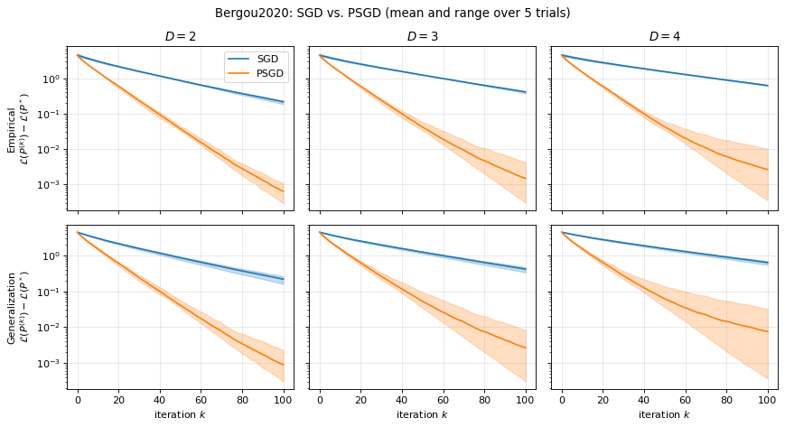
Fig. 14 Bergou2020: the optimality gap of the empirical (top) and generalization (bottom) losses.

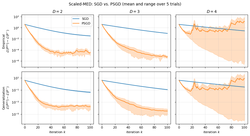
Fig. 15 Scaled-MED: the optimality gap of the empirical (top) and generalization (bottom) losses.

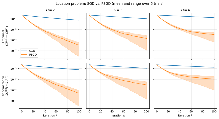
Fig. 16 Location problem: the optimality gap of the empirical (top) and generalization (bottom) losses.

The skew-MMD has no closed-form solution, so its figure shows the loss \(\mathcal L(P^{(k)})\) itself:

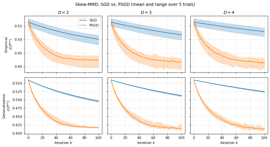
Fig. 17 Skew-MMD: the empirical (top) and generalization (bottom) losses.

PSGD decreases both losses much faster than SGD on every problem, with one exception discussed below. After 100 iterations, its optimality gap is two to five orders of magnitude smaller (e.g., \(6 \times 10^{-4}\) against \(2 \times 10^{-1}\) for Bergou2020 with \(D = 2\)), and the generalization loss follows the empirical one. The higher the degree, the slower SGD gets, because the Bernstein basis gets more ill-conditioned: the condition number of \(\Sigma\) of a Bézier triangle is 15, 56 and 210 for \(D = 2, 3, 4\). PSGD removes this dependence in its first iterations, which decrease the loss at almost the same rate for every degree, as the paper reports.

The exception is Scaled-MED with \(D = 4\): the gap of PSGD jumps up during the iterations in two of the five trials, so that its mean ends above that of SGD, although PSGD is ahead in the first 20 iterations and in the other three trials. The paper proves the convergence of minibatch PSGD for step sizes up to a bound proportional to \(1 / \lambda_{\max}(\Sigma^{-1})\), which shrinks as the degree grows (\(\lambda_{\max}(\Sigma^{-1})\) of a Bézier triangle is 90, 560 and 3150 for \(D = 2, 3, 4\)), and \(\alpha = 0.05\) is apparently beyond it here: a minibatch whose samples miss part of the triangle gets its gradient amplified along the directions where \(\Sigma\) is small. With \(\alpha = 0.03\), all five trials converge. If the loss of PSGD jumps up, decrease step_size, use step_decay="sqrt", or enlarge batch_size.

The other figures show the Pareto set and front approximated by PSGD after 100 iterations, in the trial of the median final empirical optimality gap (empirical loss for the skew-MMD), with the control points (red) and, where known, the boundary of the true Pareto set and front (dotted). For the location problem, the Pareto set lies in \(x_4 = 0\) and is drawn in \((x_1, x_2, x_3)\).

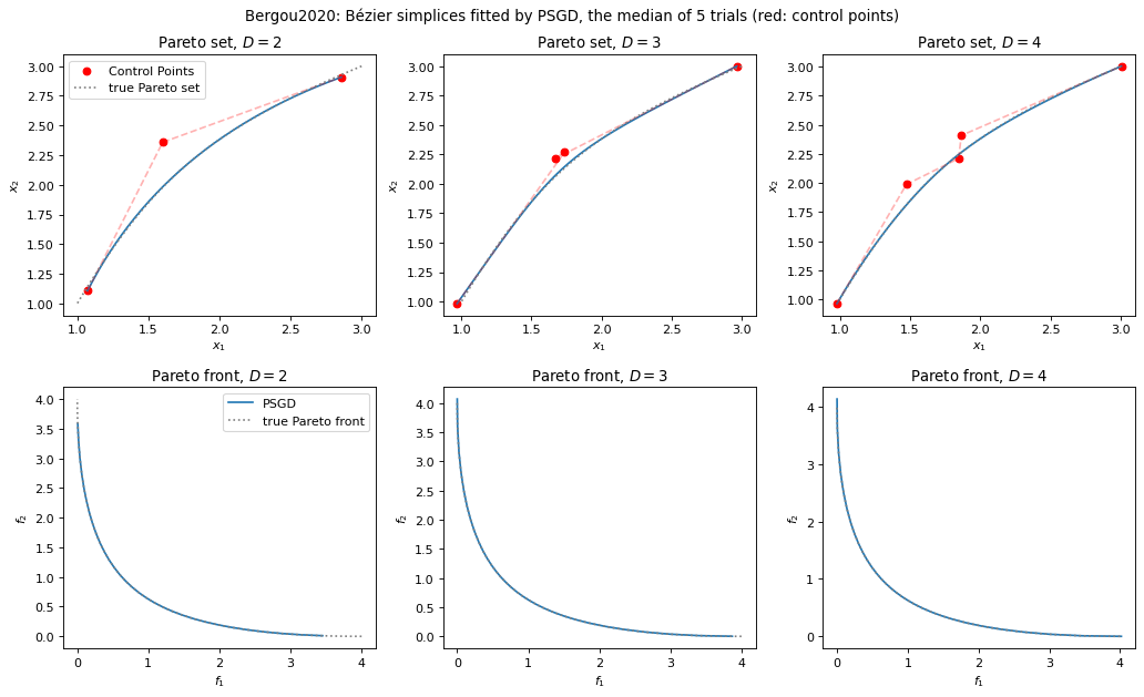
Fig. 18 Bergou2020: the approximated Pareto set (top) and front (bottom). The true ones are given by \(x_1^*(\mathbf t) = (t_1^2 + t_1 - 3) / (t_1^2 - t_1 - 1)\) and \(x_2^*(\mathbf t) = (3t_1^2 - t_1 - 3) / (t_1^2 - t_1 - 1)\).

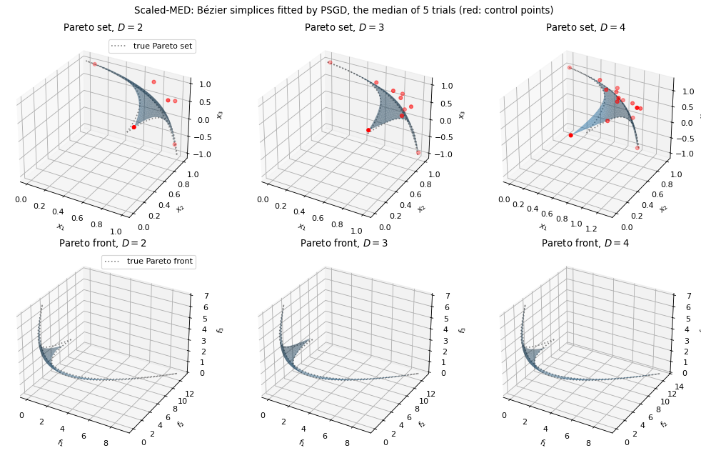
Fig. 19 Scaled-MED: the approximated Pareto set (top) and front (bottom).

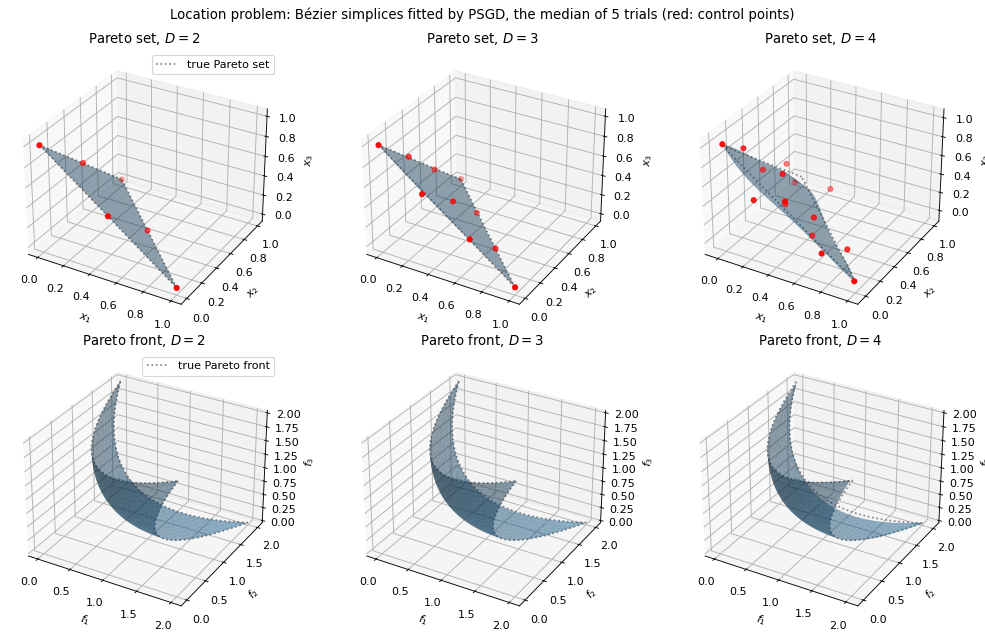
Fig. 20 Location problem: the approximated Pareto set (top) and front (bottom).

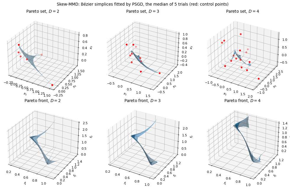
Fig. 21 Skew-MMD: the approximated Pareto set (top) and front (bottom).

On Bergou2020, the end points of the curve, which correspond to the vertices of the simplex that uniform samples of \(\mathbf t\) rarely approach, converge the slowest. On the skew-MMD, \(f_1\) is not convex (\(p_1 = e^{-1} < 1\)), so the minimizers of the linear scalarization \(\mathbf t^\top f(\mathbf x)\) need not trace the Pareto set smoothly, and the fitted surface is only a local minimizer of \(\mathcal L\); the paper uses this problem only for the convergence comparison.

The last figures correspond to Figure 4 of Hikima et al. [HKT+25]: they compare how close the approximated Pareto set gets to the true one, by the mean squared error of Section 5.3 of the paper,

\[\mathrm{MSE}(P) = \frac{1}{N} \sum_{i=1}^N \bigl\| b(\mathbf t_i \mid P) - \mathbf x^*(\mathbf t_i) \bigr\|_2^2,\]

where \(\mathbf x^*(\mathbf t)\) is the minimizer of \(\mathbf t^\top f(\mathbf x)\) given in closed form above and \(\mathbf t_1, \dots, \mathbf t_N\) are the \(N = 10{,}000\) samples of the generalization loss. It is recorded at \(P^{(0)}, \dots, P^{(K)}\) in the same callback under torch.no_grad(); at \(P^{(0)} = O\), it is the mean of \(\|\mathbf x^*(\mathbf t_i)\|_2^2\). The script draws the MSE of the location problem and Scaled-MED, as the paper does, and of Bergou2020, whose Pareto set is also known. As in the other figures, the band is the range over the 5 trials, whereas the paper shows a 95% confidence interval.

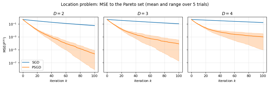
Fig. 22 Location problem: the MSE to the true Pareto set.

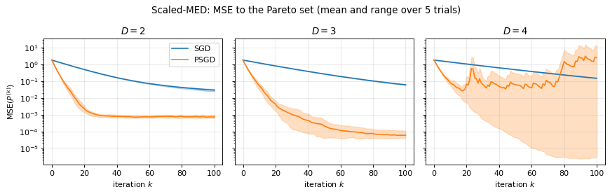
Fig. 23 Scaled-MED: the MSE to the true Pareto set.

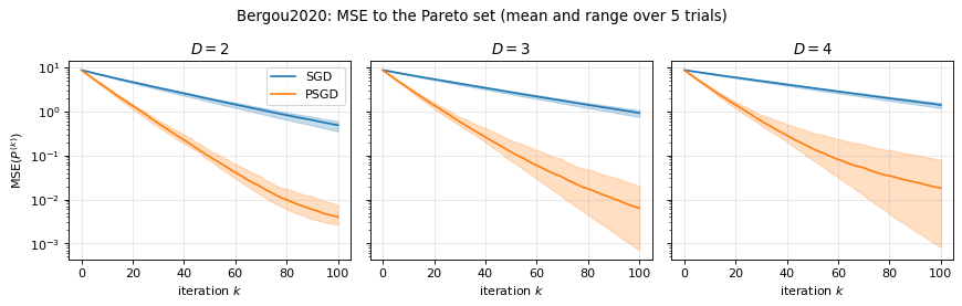
Fig. 24 Bergou2020: the MSE to the true Pareto set.

The MSE follows the optimality gap. For the location problem, \(\mathbf t^\top f(\mathbf x) = \|\mathbf x - \mathbf x^*(\mathbf t)\|_2^2 + 1 - \|\mathbf x^*(\mathbf t)\|_2^2\) on the simplex, so the MSE equals the generalization optimality gap; \(\mathbf x^*\) is linear in \(\mathbf t\) and the MSE of PSGD keeps decreasing towards zero (to \(2 \times 10^{-6}\) after 100 iterations with \(D = 2\), against \(6 \times 10^{-2}\) for SGD). For Scaled-MED and Bergou2020, \(\mathbf x^*\) is a rational function that a Bézier simplex of degree \(D\) cannot represent exactly, so even the minimizer \(P^*\) of the generalization loss has a positive MSE, which decreases with the degree (\(6 \times 10^{-4}\), \(3 \times 10^{-5}\) and \(2 \times 10^{-6}\) for Scaled-MED with \(D = 2, 3, 4\)). The MSE of PSGD for Scaled-MED with \(D = 2\) levels off near this floor after about 30 iterations, while SGD is still two orders of magnitude above it. The divergence of PSGD in two trials of Scaled-MED with \(D = 4\) discussed above shows up in the MSE as well: the mean MSE of PSGD ends at 2.6, above the 0.15 of SGD, because one trial ends at 13 and another rises from \(3 \times 10^{-4}\) to \(2 \times 10^{-3}\), whereas the other three trials end below \(10^{-3}\).