Supply Chain and Logistics Optimization
In modern supply chain management (SCM) and operations research, isolating physical material logistics from global financial flows regularly causes massive inefficiencies. Supply Chain Finance algorithms attempt to computationally integrate factory outputs, inventory storage, and monetary streams to achieve a single unified, profitable coordination strategy.
Recent operational formulations actively model this extensive corporate balancing act as a purely convex, constrained, finite-horizon Linear Quadratic Regulator (LQR) problem over discrete stages.
The optimization generally maps out three tightly competing operational objectives across the logistics network:
Where \(X_k\) represents the aggregate cash and inventory states, constrained to remain close to their targets without causing disruptive shortages, and \(U_k\) are the direct financial interventions or operational accelerations.
For manufacturing processes and logistics, abrupt disruptions in financing inputs or delivery capacities incur massive overheads, making the penalization of policy volatility (\(\|\Delta U_k\|_S^2\)) practically vital for securing stable operational margins.
Because the entire LQR overarching formulation relies exclusively on positive definite penalty matrices (\(Q, R, S \succ 0\)), the extensive supply chain network optimization mathematically remains entirely and globally strongly convex.
When corporate managers visualize these strategic relationships statically, they often suffer from disjointed discrete scenario planning. Implementing a Bézier simplex surrogate that models the multi-objective continuous terrain flawlessly allows disparate corporate departments—ranging from financial officers to warehouse managers—to visually navigate through a single, continuous interactive Pareto topology in boardroom meetings, instantly resolving the optimal, stable path for navigating market supply shocks without requiring live, intensive QP solver re-computations.
Numerical Experiments
We demonstrate Bézier simplex fitting on a two-objective inventory LQR problem balancing state deviation against policy volatility over a horizon of \(H = 5\) periods.
Problem Setup:
Ordering decisions: \(U = [u_0, u_1, u_2, u_3, u_4] \in \mathbb{R}^5\)
Inventory dynamics: \(x(k+1) = x(k) + u(k)\), \(x(0) = 0\), target \(x^* = 1\)
Competing objectives:
Experiment Procedure:
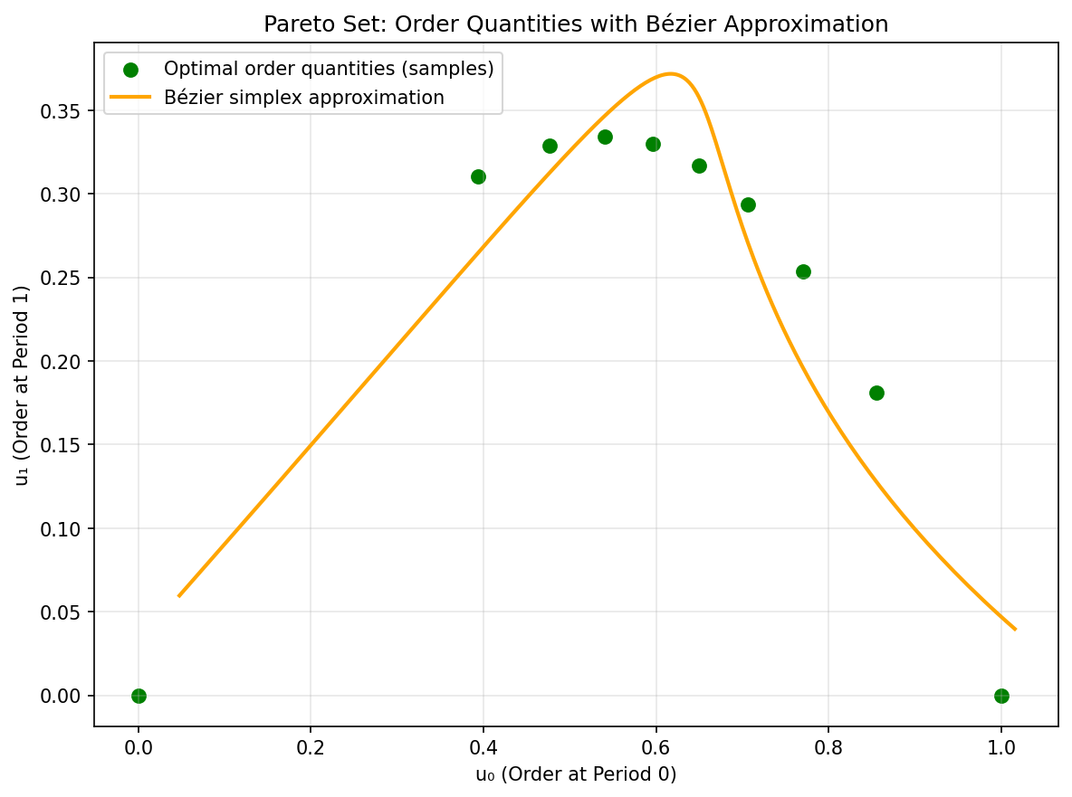
Sample 10 weight vectors \(w = (w_1, w_2)\) on the 1-simplex from \((1,0)\) to \((0,1)\).
For each \(w\), solve \(U^*(w) = \arg\min_U [w_1 f_1(U) + w_2 f_2(U)]\) using L-BFGS-B.
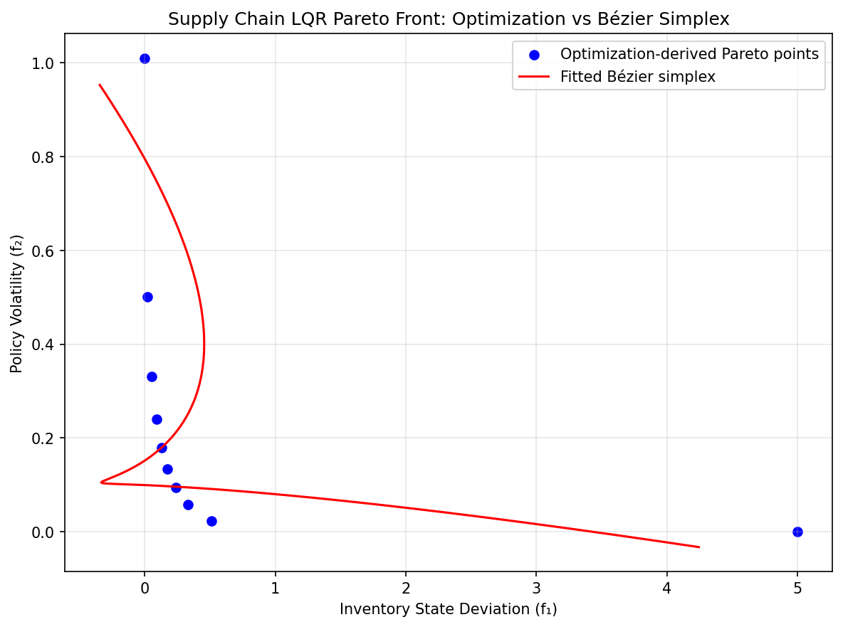
Collect the Pareto front points \((f_1(U^*(w)), f_2(U^*(w)))\).
Fit a degree-3 Bézier simplex to the weight–objective pairs.
Visualize the fitted Bézier curve against the optimization-derived Pareto front.
|
|
Pareto set. |
Pareto front. |
The complete example script is available at examples/generate_supply_chain_pareto.py.