Facility Location and Continuous Approximations
Strongly convex multi-objective frameworks naturally accommodate classic spatial, physical, and logistics challenges. For instance, urban planning and supply chain optimization frequently involve determining the optimal spatial coordinates for physical facilities (e.g., warehouses, hospitals, or transit hubs) to mutually minimize the travel distances to several distributed demand points.
In such Weber-type facility location problems, when evaluating trade-offs using squared Euclidean distances, the formulation becomes a simultaneous minimization of multiple objectives:
Where \(x\) represents the facility location and \(a_k\) represents the fixed locations of the demand segments. The modulus-2 strong convexity of each distance objective, since the Hessian is identically \(2I \succ 0\), translates directly into a simplicial Pareto set topology [HHI+20]. Since the objectives are all strongly convex, the Pareto set forms a continuous simplex in the decision space.
Likewise, in engineering design optimizing for structural compliance or minimum energy, the objectives inherently manifest as positive-definite quadratic costs. The strong convexity ensures that descent methods, such as the multi-objective Newton method, achieve superlinear or even quadratic local convergence along the Pareto front [FGranaDS09].
These properties are explicitly leveraged by Adaptive Weighted Sum (AWS) methods in structural multidisciplinary optimization, where successive boundary-constrained strongly-convex QPs smoothly and uniformly map the Pareto front [dWK]. Even in complex biological systems, such as competitive Lotka-Volterra models, transformations of the quadratic interaction terms yield strongly convex models that exhibit identically stable simplicial Pareto behavior.
Approximating these Pareto fronts with a Bézier simplex yields a completely continuous, analytic structural location map. Planners and decision-makers are empowered to visually and analytically slide trade-off priorities—such as selectively favoring certain demand hubs—to determine the optimal coordinates seamlessly, without needing to re-solve the spatial optimization from scratch.
Numerical Experiments
To demonstrate the scalability of Bézier simplex fitting across different numbers of objectives, we generate Pareto front samples for two, three, and four objectives by solving weighted sums of convex squared-distance objectives.
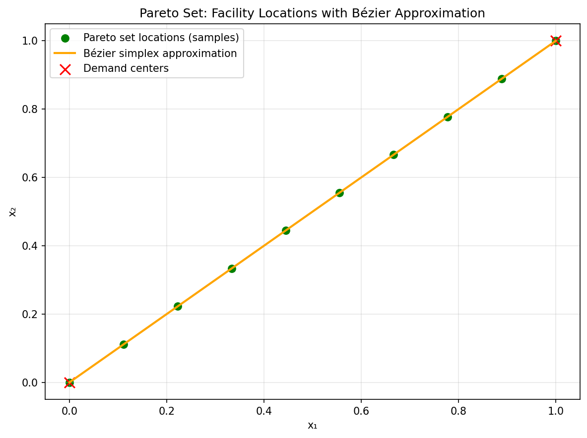
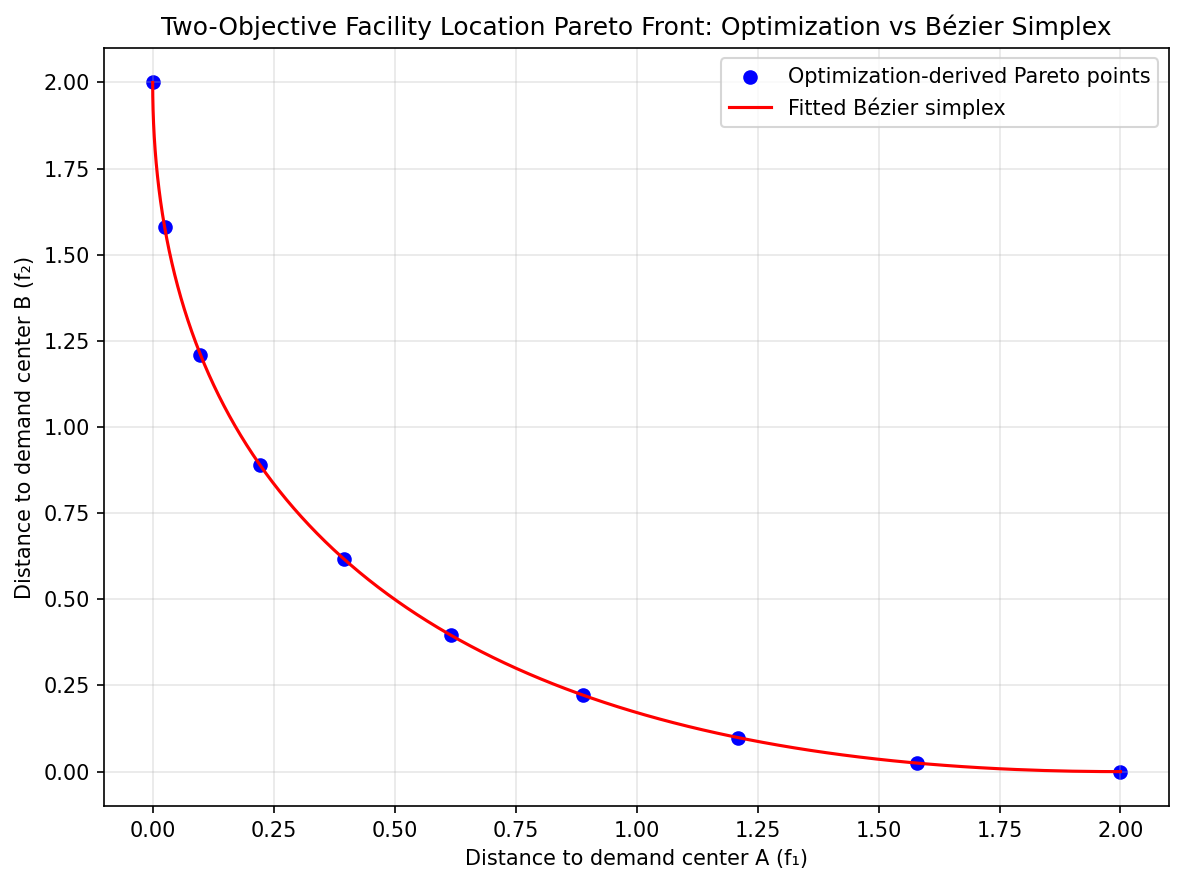
Two Objectives: We consider two demand centers at \(a_1=(0,0)\) and \(a_2=(1,1)\), with objectives \(f_1(x) = \lVert x - a_1\rVert^2\) and \(f_2(x) = \lVert x - a_2\rVert^2\). The weighted objective \(f(x, w) = w_1 f_1(x) + w_2 f_2(x)\) is strongly convex. We sample 10 weights and fit a degree-3 Bézier simplex.
|
|
Pareto set (2-obj). |
Pareto front (2-obj). |
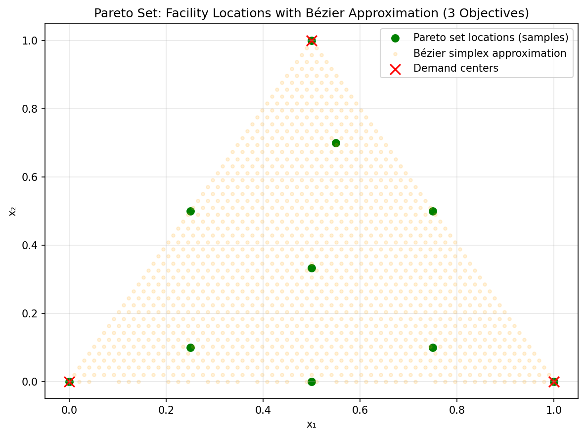
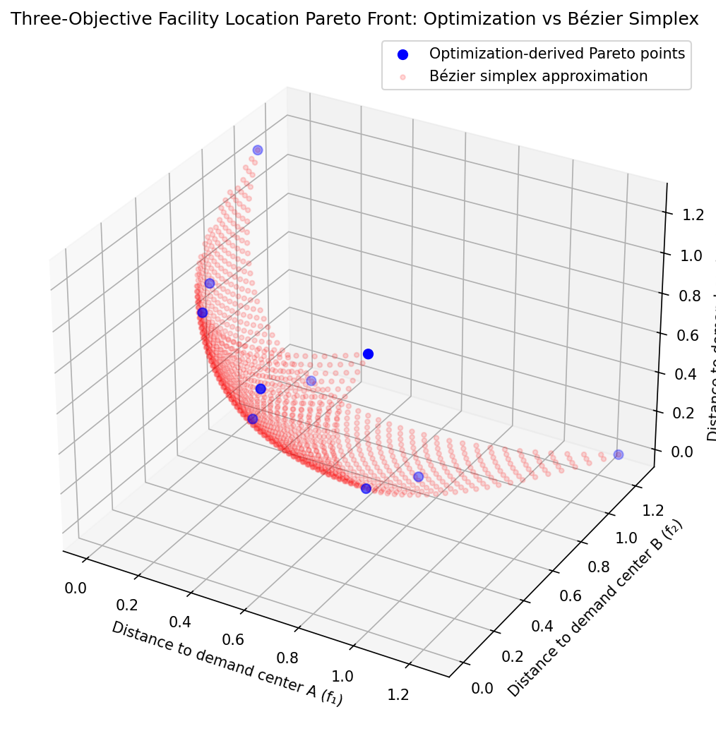
Three Objectives: We consider three demand centers at \(a_1=(0,0)\), \(a_2=(1,0)\), and \(a_3=(0.5,1)\), with \(f_k(x) = \lVert x - a_k\rVert^2\) for each \(k\). The weighted objective is \(f(x, w) = w_1 f_1(x) + w_2 f_2(x) + w_3 f_3(x)\). We sample 10 weight vectors on the 3-simplex and fit a degree-3 Bézier simplex.
|
|
Pareto set (3-obj). |
Pareto front (3-obj). |
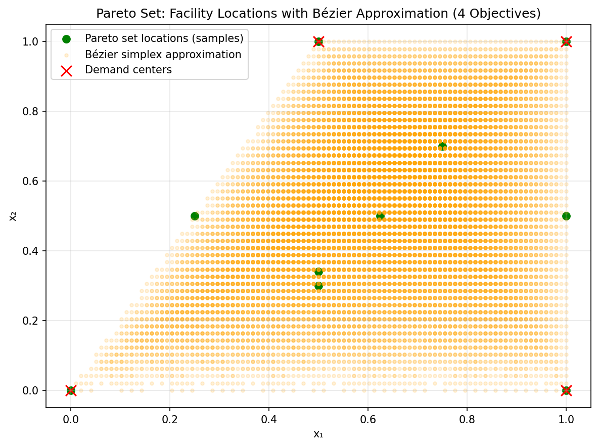
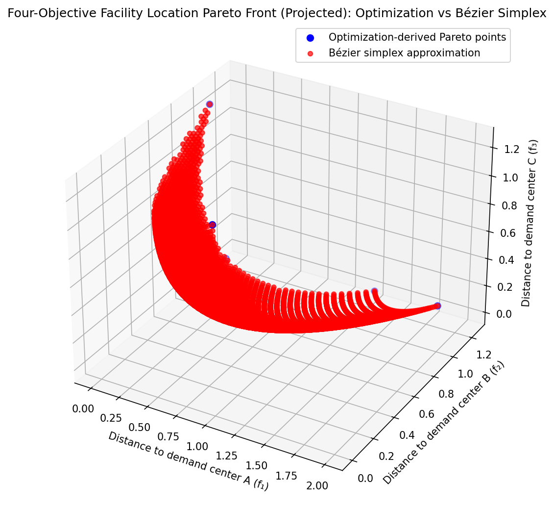
Four Objectives: We add a fourth demand center at \(a_4=(1,1)\), with \(f_4(x) = \lVert x - a_4\rVert^2\). The weighted objective is \(f(x, w) = w_1 f_1(x) + w_2 f_2(x) + w_3 f_3(x) + w_4 f_4(x)\). We sample 10 weight vectors on the 3-simplex and fit a degree-2 Bézier simplex. For visualization, we project to 3D by plotting \(f_1, f_2, f_3\).
|
|
Pareto set (4-obj). |
Pareto front (4-obj). |
These examples confirm that Bézier simplex fitting accurately approximates multi-objective facility location trade-offs from actual optimization, scaling effectively to higher dimensions. The complete code for the two-, three-, and four-objective experiments is available in examples/generate_facility_location_pareto_2obj.py, examples/generate_facility_location_pareto_3obj.py, and examples/generate_facility_location_pareto_4obj.py, respectively.