Communication Systems and Routing

In modern communication networks, backbone infrastructure must dynamically adjust routes to accommodate wildly fluctuating traffic demands from streaming services, cloud computing, and IoT devices. Traffic Engineering (TE) utilizing Model Predictive Control (MPC) resolves these complex allocations but faces competing demands: operators must route packets efficiently to strictly avoid bandwidth congestion, yet they must also suppress erratic, sudden changes to the routing policies to maintain overall network stability.

This routing challenge is frequently framed as a strongly convex multi-objective optimization problem over a predictive time horizon.

\[\begin{split}\text{Congestion Excess: } & f_1(R) = \sum_{k=t+1}^{t+h} \|\zeta(k)\|_2^2 \\ \text{Route Volatility: } & f_2(R) = \sum_{k=t+1}^{t+h} \|\Delta R(k)\|_2^2\end{split}\]

Where \(R(k)\) is the routing allocation matrix at time step \(k\), \(\zeta(k)\) represents the bandwidth excess above target capacity, and \(\Delta R(k)\) denotes the modifications applied to the traffic routing.

Simultaneously minimizing both objectives heavily relies on strong convexity. Even if the network flow constraints are piece-wise linear or broadly just convex, the explicit \(L_2\) penalty on the route changes (\(\|\Delta R(k)\|_2^2\)) injects a mathematically strict positive-definite curvature into the optimization landscape. This uniformly bounds the Hessian away from zero, enforcing the strong convexity of the routing matrix modifications.

For real-time network controllers, instantly reacting to traffic bursts while balancing these trade-offs using standard Quadratic Programming solvers at every microsecond is computationally prohibitive. By fitting a Bézier simplex to the Pareto front of the sub-games, operators unlock an instantaneous, purely arithmetic continuous mapping of the exact trade-offs between congestion and routing modifications. The network can then dynamically, and safely, slide along the Pareto front using continuous polynomial evaluations instead of repeatedly executing heavy optimization loops, ensuring uninterrupted low-latency services.

Numerical Experiments

To demonstrate the effectiveness of Bézier simplex fitting for approximating Pareto fronts in communication systems, we conducted an experiment using actual optimization to generate the Pareto front samples.

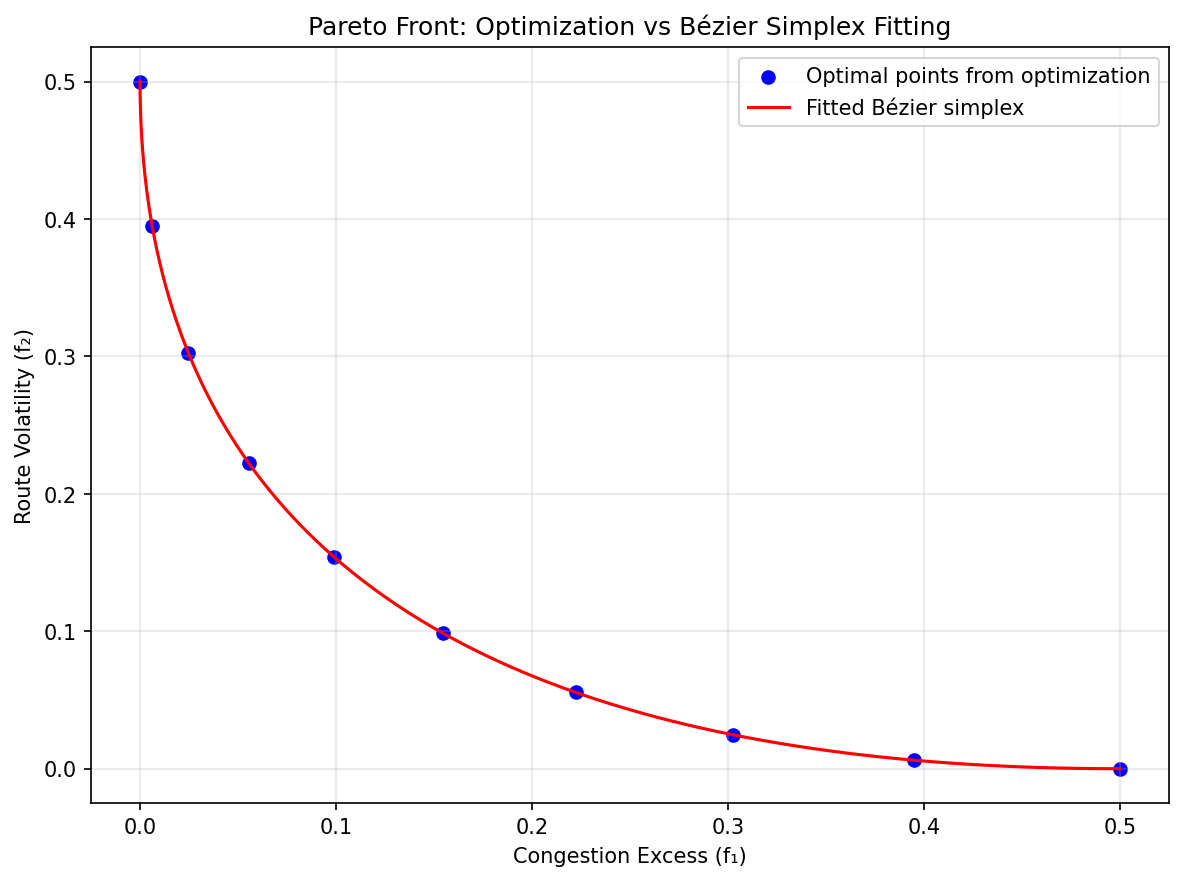
Problem Setup: We define a simplified routing optimization problem with two objectives: - Congestion Excess: \(f_1(x) = x_1^2 + x_2^2\) - Route Volatility: \(f_2(x) = (x_1 - 0.5)^2 + (x_2 - 0.5)^2\)

where \(x = (x_1, x_2)\) represents routing allocations. The weighted objective function \(f(x, w) = w_1 f_1(x) + w_2 f_2(x)\) is strongly convex.

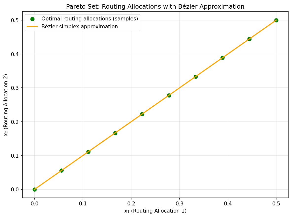
Experiment Procedure: 1. Sample 10 weights \(w\) from \((1,0)\) to \((0,1)\). 2. For each \(w\), solve \(x^*(w) = \arg\min_x f(x, w)\) using L-BFGS optimization. 3. Collect the Pareto front points \((f_1(x^*(w)), f_2(x^*(w)))\). 4. Fit a degree-3 Bézier simplex to the weight-objective value pairs. 5. Visualize the fitted Bézier approximation against the optimization-derived Pareto front.

Pareto set.	Pareto front.

This experiment shows that Bézier simplex fitting can accurately approximate Pareto fronts derived from actual optimization, enabling real-time trade-off evaluation in communication network routing.

Three-Objective Extension

To demonstrate multi-objective scalability, we also consider a three-objective routing problem:

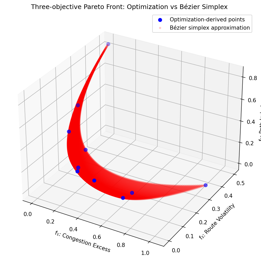
• \(f_1(x) = x_1^2 + x_2^2\)

• \(f_2(x) = (x_1 - 0.5)^2 + (x_2 - 0.5)^2\)

• \(f_3(x) = 0.8\left((x_1 - 1.0)^2 + (x_2 - 0.2)^2\right)\)

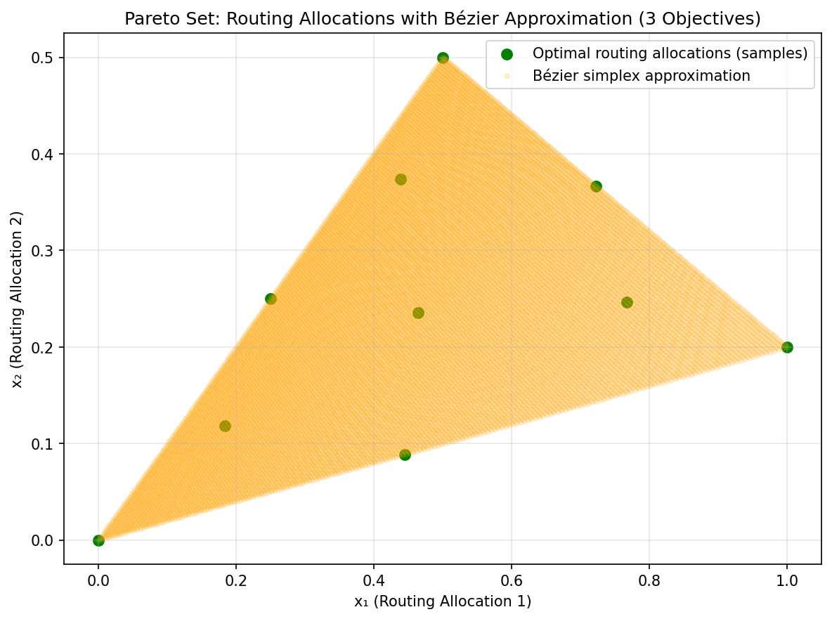
The weighted objective \(f(x, w) = w_1 f_1(x) + w_2 f_2(x) + w_3 f_3(x)\) is strongly convex. We sampled 10 weight vectors on the 2-simplex, solved each weighted optimization with L-BFGS, and fitted a degree-3 Bézier simplex to the resulting objective triples.

Pareto set.	Pareto front.

The fit achieves nearly zero training error on the sampled Pareto points, demonstrating that Bézier simplex fitting can accurately approximate three-objective trade-offs from actual optimization.

The complete code for the two-objective and three-objective experiments is available in examples/generate_communication_pareto.py and examples/generate_communication_pareto_3obj.py, respectively.