Objective minimization

Regression and differentiable objective minimization are separate problems:

import torch
from torch_bsf import BezierSpace, BezierModel, minimize, PreconditionedSGD
from torch_bsf.optimization import linear_scalarization

space = BezierSpace.simplex(1, degree=2)
initial = BezierModel(space, torch.zeros(space.n_controls, 1, dtype=torch.float64))
def objectives(x):
    return torch.cat([(x-1)**2, (x+1)**2], dim=1)
result = minimize(initial, linear_scalarization(objectives), seed=7,
                  method=PreconditionedSGD(max_iter=300, gradient_tolerance=1e-6))

loss(predicted_values, points) returns one differentiable scalar per row. minimize copies the initial model. Exact domain Gram preconditioning, minibatches, quadratic penalties and explicit fixed controls are available. The method does not require Lightning. Float16/bfloat16 initial models are copied and promoted to float32 on the same device for basis evaluation, gradients and metric solves. The returned model then has float32 coefficients.

History records pre-update losses and gradient norms. Iteration-budget exhaustion and callback stops do not establish convergence. Only a checked full-sample gradient tolerance or all-fixed problem yields success=True. The final objective is evaluated on the complete fixed sample set.

The algorithm

Let \(f = (f_1, \ldots, f_M): \mathbb R^L \to \mathbb R^M\) be the objectives and \(b(\mathbf t \mid P) = P^\top \mathbf z(\mathbf t)\) a Bézier simplex of degree \(D\) on \(\Delta^{M-1}\), where \(\mathbf z(\mathbf t)\) is the vector of the Bernstein basis polynomials. The paper minimizes the linear scalarization weighted by the parameter itself, averaged over the simplex:

\[\mathcal L(P) = \mathbb E_{\mathbf t \sim U(\Delta^{M-1})}\bigl[\mathbf t^\top f(b(\mathbf t \mid P))\bigr].\]

For strongly convex objectives, the minimizer of \(\mathbf t^\top f(\mathbf x)\) traces the whole Pareto set as \(\mathbf t\) moves on the simplex, so the minimizer of \(\mathcal L\) approximates the Pareto set, parametrized by the weight.

The expectation is replaced by the mean over \(n\) fixed samples \(\mathbf t_1, \ldots, \mathbf t_n\), and the control points are updated on minibatches \(B\) of them:

\[P^{(k+1)} = P^{(k)} - \alpha_k \Sigma^{-1} \nabla \mathcal L_B(P^{(k)}), \qquad \Sigma = \mathbb E_{\mathbf t \sim U(\Delta^{M-1})}\bigl[\mathbf z(\mathbf t)\,\mathbf z(\mathbf t)^\top\bigr].\]

The preconditioner \(\Sigma^{-1}\) turns the step into the one that minimizes the linearized loss plus \(\frac{1}{2\alpha_k}\mathbb E_{\mathbf t}\|b(\mathbf t \mid P) - b(\mathbf t \mid P^{(k)})\|^2\): it measures how far the surface moves rather than how far its control points move. The paper proves that this converges faster than plain SGD (\(\Sigma = I\)), whose steps are distorted by the ill-conditioning of the Bernstein basis. gram_matrix() computes \(\Sigma\) exactly, for the configured cell distribution.

Historical benchmark figures

The figures below were generated before the unified API migration. They illustrate the research problems and are not performance measurements of this release. The migrated script can generate fresh figures and metrics.

Benchmarks: SGD vs. PSGD

The script examples/sgd_benchmarks.py reproduces the experiments of Section 5 of Hikima et al. [HKT+25] with minimize(), comparing plain SGD (preconditioner="none") with the preconditioned SGD of the paper (PSGD, preconditioner="gram"). The problems are implemented from their definitions in the paper:

• Bergou2020 [BDK21] (\(M = 2\), \(L = 2\)): \(f_1(\mathbf x) = (x_1 - 1)^2 + (x_1 - x_2)^2\) and \(f_2(\mathbf x) = (x_2 - 3)^2 + (x_1 - x_2)^2\).

• Scaled-MED (\(M = 3\), \(L = 3\)): \(f_1(\mathbf x) = x_1^2 + 3(x_2 - 1)^2 + 2(x_3 - 1)^2\), \(f_2(\mathbf x) = 2(x_1 - 1)^2 + x_2^2 + 3(x_3 - 1)^2\) and \(f_3(\mathbf x) = 3(x_1 - 1)^2 + 2(x_2 - 1)^2 + (x_3 + 1)^2\).

• Skew-MMD (\(M = 3\), \(L = 3\)): \(f_i(\mathbf x) = \|A_i(\mathbf x - \mathbf e_i)\|_2^{p_i}\) with \(A_1 = \operatorname{diag}(3/5, 4/5, 4/5)\), \(A_2 = \operatorname{diag}(4/5, 3/5, 4/5)\), \(A_3 = \operatorname{diag}(4/5, 4/5, 3/5)\) and \(p_i = \exp(2(i - 1)/(M - 1) - 1)\).

• Skew-MMD, transformed (\(M = 3\), \(L = 3\), not in the paper): \(g_i(\mathbf x) = f_i(\mathbf x)^{2/p_i} = \|A_i(\mathbf x - \mathbf e_i)\|_2^2\) with the \(f_i\) of the skew-MMD, which has the same Pareto set (see Non-convex objectives: transforming the skew-MMD).

• Location problem (\(M = 3\), \(L = 4\)): \(f_i(\mathbf x) = \|\mathbf x - \mathbf e_i\|_2^2\), whose Pareto set is the triangle spanned by \(\mathbf e_1, \mathbf e_2, \mathbf e_3\).

The settings are those of the paper: \(P_0 = O\), \(n = 100\) samples, minibatches of \(m = 20\), \(K = 100\) iterations with the constant step size \(\alpha = 0.05\), the degrees \(D \in \{2, 3, 4\}\), and 5 trials with different samples, SGD and PSGD sharing the samples of a trial. The losses are recorded with callback as in the explicit optimizer callback: the empirical loss on the \(n\) samples and the generalization loss on 10,000 other samples. The script plots with matplotlib and SciPy, which the plot extra installs. In a clone of the repository, run

pip install -e ".[plot]"
python examples/sgd_benchmarks.py

to write the figures below to docs/_static/; it takes less than a minute on a CPU.

For all the problems but the skew-MMD, the objectives are quadratic, so \(\mathcal L(P)\) is a quadratic function of the control points, and the script computes its minimizer \(P^*\) over the Bézier simplices of degree \(D\) exactly (by Newton’s method, on the \(n\) samples for the empirical loss and on the 10,000 samples for the generalization loss). The figures show the optimality gap \(\mathcal L(P^{(k)}) - \mathcal L(P^*)\), the mean over the trials as a line and the range as a band:

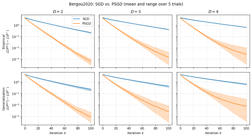
Fig. 18 Bergou2020: the optimality gap of the empirical (top) and generalization (bottom) losses.

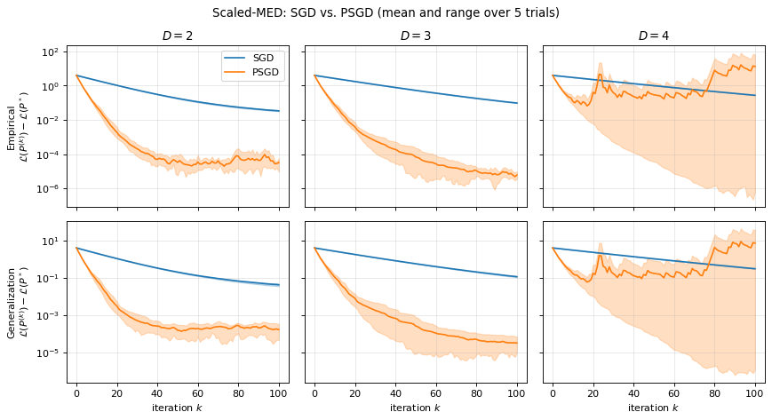
Fig. 19 Scaled-MED: the optimality gap of the empirical (top) and generalization (bottom) losses.

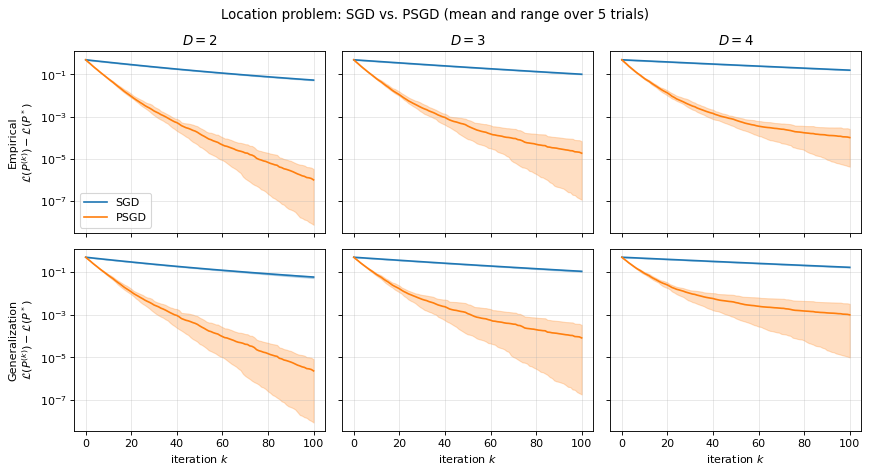
Fig. 20 Location problem: the optimality gap of the empirical (top) and generalization (bottom) losses.

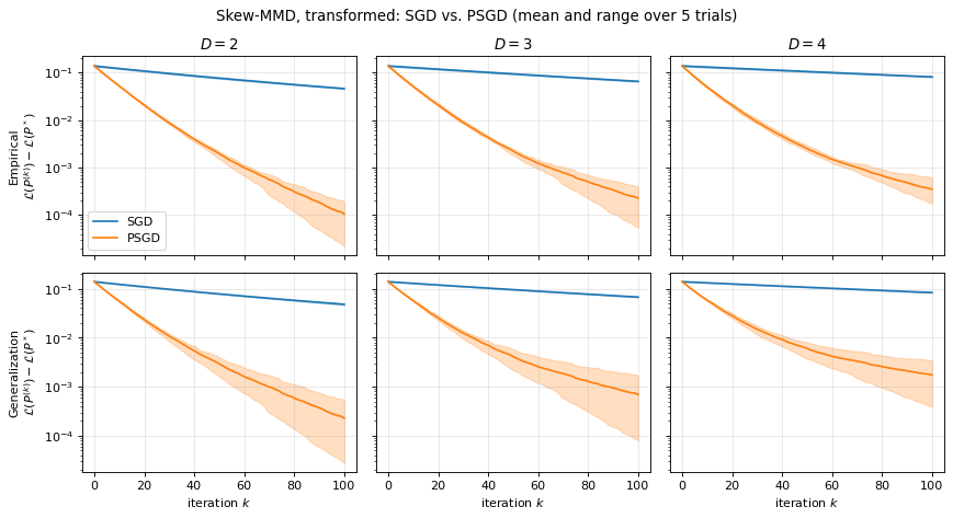
Fig. 21 Skew-MMD, transformed: the optimality gap of the empirical (top) and generalization (bottom) losses.

The loss of the skew-MMD is not convex and its minimizer has no closed form, so its figure shows the loss \(\mathcal L(P^{(k)})\) itself:

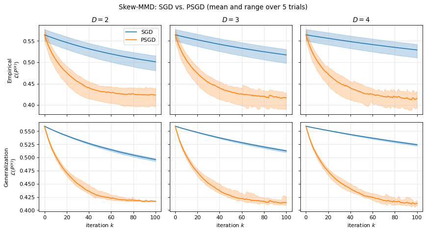
Fig. 22 Skew-MMD: the empirical (top) and generalization (bottom) losses.

PSGD decreases both losses much faster than SGD on every problem, with one exception discussed below. After 100 iterations, its optimality gap is two to five orders of magnitude smaller (e.g., \(6 \times 10^{-4}\) against \(2 \times 10^{-1}\) for Bergou2020 with \(D = 2\)), and the generalization loss follows the empirical one. The higher the degree, the slower SGD gets, because the Bernstein basis gets more ill-conditioned: the condition number of \(\Sigma\) of a Bézier triangle is 15, 56 and 210 for \(D = 2, 3, 4\). PSGD removes this dependence in its first iterations, which decrease the loss at almost the same rate for every degree, as the paper reports.

The exception is Scaled-MED with \(D = 4\): the gap of PSGD jumps up during the iterations in two of the five trials, so that its mean ends above that of SGD, although PSGD is ahead in the first 20 iterations and in the other three trials. The paper proves the convergence of minibatch PSGD for step sizes up to a bound proportional to \(1 / \lambda_{\max}(\Sigma^{-1})\), which shrinks as the degree grows (\(\lambda_{\max}(\Sigma^{-1})\) of a Bézier triangle is 90, 560 and 3150 for \(D = 2, 3, 4\)), and \(\alpha = 0.05\) is apparently beyond it here: a minibatch whose samples miss part of the triangle gets its gradient amplified along the directions where \(\Sigma\) is small. With \(\alpha = 0.03\), all five trials converge. If the loss of PSGD jumps up, decrease step_size, use step_decay="sqrt", or enlarge batch_size.

The other figures show the Pareto set and front approximated by PSGD after 100 iterations, in the trial of the median final empirical optimality gap (empirical loss for the skew-MMD), with the control points (red) and the boundary of the true Pareto set and front (dotted). For the location problem, the Pareto set lies in \(x_4 = 0\) and is drawn in \((x_1, x_2, x_3)\).

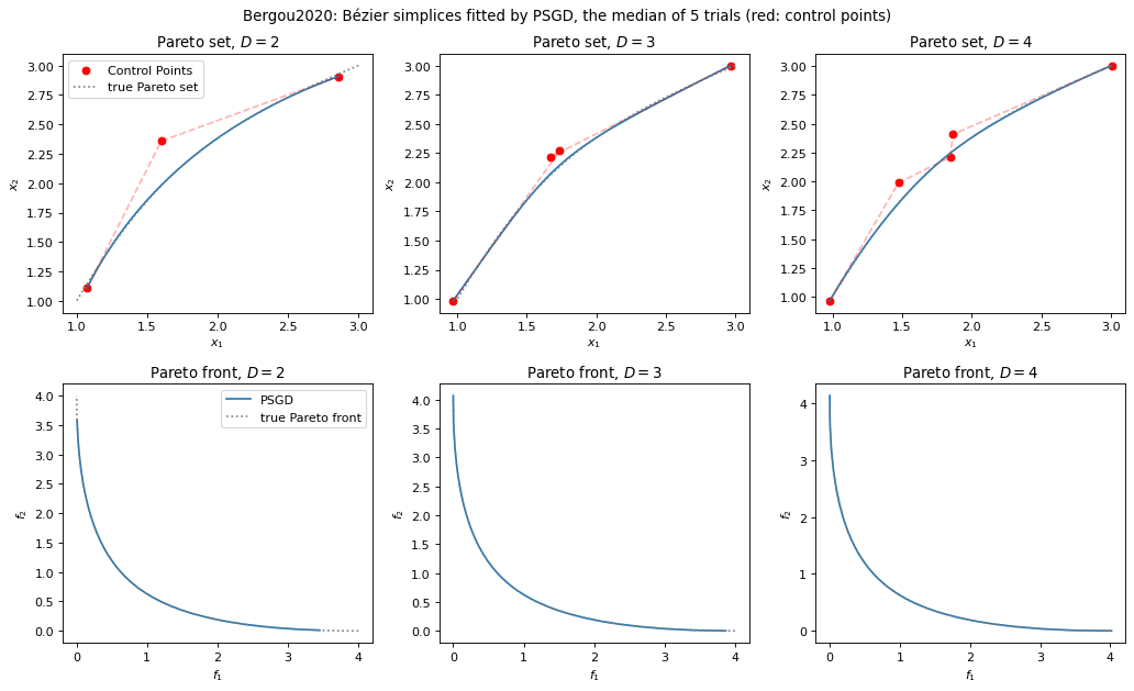
Fig. 23 Bergou2020: the approximated Pareto set (top) and front (bottom). The true ones are given by \(x_1^*(\mathbf t) = (t_1^2 + t_1 - 3) / (t_1^2 - t_1 - 1)\) and \(x_2^*(\mathbf t) = (3t_1^2 - t_1 - 3) / (t_1^2 - t_1 - 1)\).

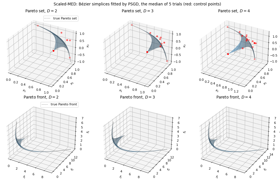
Fig. 24 Scaled-MED: the approximated Pareto set (top) and front (bottom).

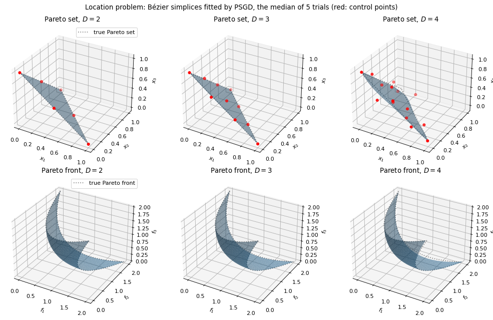
Fig. 25 Location problem: the approximated Pareto set (top) and front (bottom).

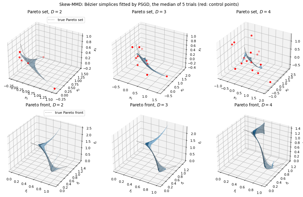
Fig. 26 Skew-MMD: the approximated Pareto set (top) and front (bottom).

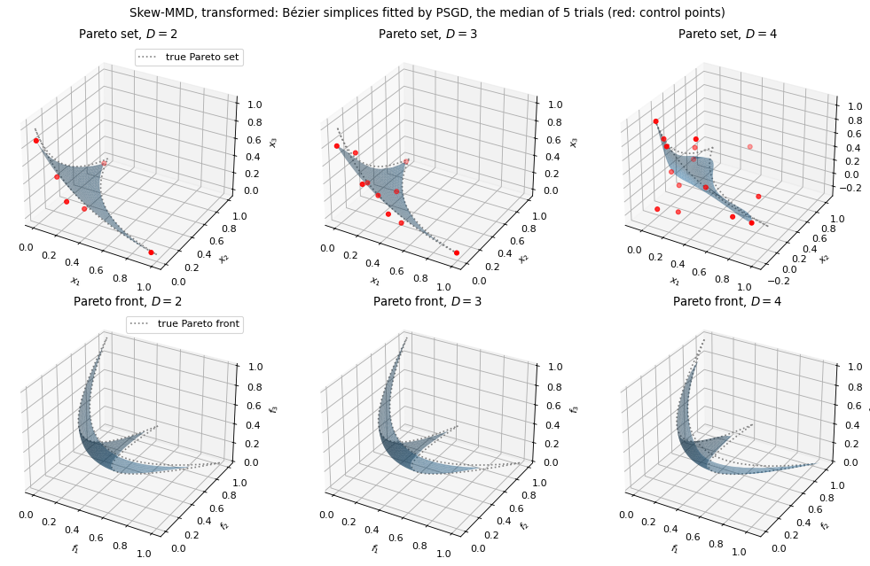
Fig. 27 Skew-MMD, transformed: the approximated Pareto set (top) and front of \(g\) (bottom).

On Bergou2020, the end points of the curve, which correspond to the vertices of the simplex that uniform samples of \(\mathbf t\) rarely approach, converge the slowest. On the skew-MMD, the fitted surface leaves the true Pareto set, whereas on its transform it follows it; see Non-convex objectives: transforming the skew-MMD.

The last figures correspond to Figure 4 of Hikima et al. [HKT+25]: they compare how close the approximated Pareto set gets to the true one, by the mean squared error of Section 5.3 of the paper,

\[\mathrm{MSE}(P) = \frac{1}{N} \sum_{i=1}^N \bigl\| b(\mathbf t_i \mid P) - \mathbf x^*(\mathbf t_i) \bigr\|_2^2,\]

where \(\mathbf x^*(\mathbf t)\) is the minimizer of \(\mathbf t^\top f(\mathbf x)\) given in closed form above and \(\mathbf t_1, \dots, \mathbf t_N\) are the \(N = 10{,}000\) samples of the generalization loss. It is recorded at \(P^{(0)}, \dots, P^{(K)}\) in the same callback under torch.no_grad(); at \(P^{(0)} = O\), it is the mean of \(\|\mathbf x^*(\mathbf t_i)\|_2^2\). The script draws the MSE of the location problem and Scaled-MED, as the paper does, and of Bergou2020 and the transformed skew-MMD, whose Pareto sets are also known. As in the other figures, the band is the range over the 5 trials, whereas the paper shows a 95% confidence interval.

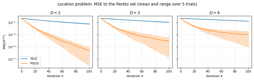
Fig. 28 Location problem: the MSE to the true Pareto set.

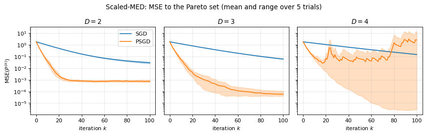
Fig. 29 Scaled-MED: the MSE to the true Pareto set.

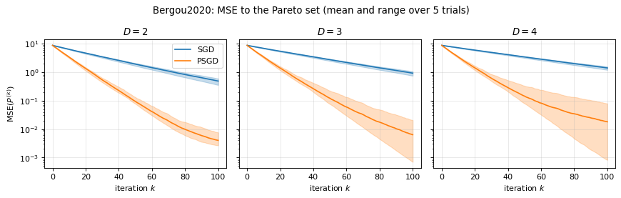
Fig. 30 Bergou2020: the MSE to the true Pareto set.

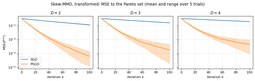
Fig. 31 Skew-MMD, transformed: the MSE to the true Pareto set.

The MSE follows the optimality gap. For the location problem, \(\mathbf t^\top f(\mathbf x) = \|\mathbf x - \mathbf x^*(\mathbf t)\|_2^2 + 1 - \|\mathbf x^*(\mathbf t)\|_2^2\) on the simplex, so the MSE equals the generalization optimality gap; \(\mathbf x^*\) is linear in \(\mathbf t\) and the MSE of PSGD keeps decreasing towards zero (to \(2 \times 10^{-6}\) after 100 iterations with \(D = 2\), against \(6 \times 10^{-2}\) for SGD). For Scaled-MED and Bergou2020, \(\mathbf x^*\) is a rational function that a Bézier simplex of degree \(D\) cannot represent exactly, so even the minimizer \(P^*\) of the generalization loss has a positive MSE, which decreases with the degree (\(6 \times 10^{-4}\), \(3 \times 10^{-5}\) and \(2 \times 10^{-6}\) for Scaled-MED with \(D = 2, 3, 4\)). The MSE of PSGD for Scaled-MED with \(D = 2\) levels off near this floor after about 30 iterations, while SGD is still two orders of magnitude above it. The divergence of PSGD in two trials of Scaled-MED with \(D = 4\) discussed above shows up in the MSE as well: the mean MSE of PSGD ends at 2.6, above the 0.15 of SGD, because one trial ends at 13 and another rises from \(3 \times 10^{-4}\) to \(2 \times 10^{-3}\), whereas the other three trials end below \(10^{-3}\).

Non-convex objectives: transforming the skew-MMD

On the skew-MMD, \(f_1\) is not convex (\(p_1 = e^{-1} < 1\)), and the linear scalarization does not trace its Pareto set: the paper uses this problem only for the convergence comparison. Its Pareto set is known all the same. An increasing transform \(h_i\) of each objective does not change which points dominate which, so the objectives \(h_i(f_i)\) have the same Pareto set as \(f_i\). The objectives of the skew-MMD are \(f_i = g_i^{p_i / 2}\) with the strongly convex quadratics \(g_i(\mathbf x) = \|A_i(\mathbf x - \mathbf e_i)\|_2^2\), so \(h_i(y) = y^{2/p_i}\) turns them into \(g_i\), whose linear scalarization has the minimizer

\[x_l^*(\mathbf t) = \frac{t_l a_{l,l}^2}{\sum_{i=1}^M t_i a_{i,l}^2}, \qquad l = 1, \ldots, L,\]

where \(a_{i,l}\) are the diagonal entries of \(A_i\). As \(\mathbf t\) moves on the simplex, \(\mathbf x^*(\mathbf t)\) traces the Pareto set of both \(f\) and \(g\), and the script draws it as the true Pareto set of both problems. On the original objectives, the global minimizer of \(\mathbf t^\top f(\mathbf x)\) collapses to the vertex \(\mathbf e_1\) for 28% of the uniform weights and to \(\mathbf e_2\) for 16%, so the linear scalarization reaches only part of the Pareto set and jumps between its parts. With \(g\), the loss is quadratic in the control points, as for the other problems: the convergence analysis of the paper applies, and the optimality gap and the MSE can be computed.

The two parametrizations differ, so the script compares them by the mean squared distance from the fitted surface to the Pareto set, \(\frac{1}{N}\sum_{i=1}^N \min_{\mathbf x \in X^*} \|b(\mathbf t_i \mid P) - \mathbf x\|_2^2\), on the first \(N = 1{,}000\) samples of the generalization loss, where \(X^*\) is the image of a fine grid of the simplex under \(\mathbf x^*\). It prints the mean over the 5 trials after 100 iterations:

Degree	Skew-MMD, PSGD	Skew-MMD, transformed, PSGD
\(D = 2\)	\(2.3 \times 10^{-3}\)	\(9.3 \times 10^{-5}\)
\(D = 3\)	\(2.0 \times 10^{-3}\)	\(2.3 \times 10^{-4}\)
\(D = 4\)	\(2.7 \times 10^{-3}\)	\(8.1 \times 10^{-4}\)

The transform brings the surface 3 to 25 times closer to the Pareto set; the higher degrees have not converged in 100 iterations yet (see the optimality gap above). To fit a model to the Pareto set of objectives that are increasing functions of convex ones, pass the transformed objectives to linear_scalarization():

p = torch.exp(torch.arange(3.0) - 1)  # the powers p_i of the skew-MMD

def transformed(x):
    return skew_mmd(x) ** (2 / p)  # h_i(f_i) = f_i^(2 / p_i)

loss = linear_scalarization(transformed)

The model is then parametrized by the weights of \(h(f)\) instead of those of \(f\). Where \(f_i\) vanishes, as at \(\mathbf x = \mathbf e_i\) here, the gradient of the composition may be undefined; write \(g_i\) directly instead, as the script does. A Chebyshev scalarization \(\max_i t_i f_i(\mathbf x)\) also reaches every Pareto point of a non-convex problem, but its minimizer stays on the boundary of the Pareto set for a whole band of weights near the boundary of the simplex, a kink that a Bézier simplex of low degree fits poorly.

A practical optimization workflow

Use objective minimization when the desired response is defined by a differentiable cost rather than paired input/output observations. For example, a model may map preference weights to decision vectors, and the cost is the weighted sum of several decision objectives. If you already have target output values and want ordinary quadratic regression, use fit instead. Direct least squares avoids learning-rate tuning for that linear problem.

Before running a long optimization, evaluate the loss at a small point batch and verify its output shape. loss(values, points) must return one finite scalar per point, not a mean over the whole batch or one loss per output. Retaining row losses allows the optimizer to sample minibatches consistently. Use PyTorch operations throughout; converting predicted values to NumPy or calling .item() inside the loss detaches the gradient path.

The following scalarized problem has an analytic solution. Its decision variable is one-dimensional and its two objectives are squared distances to one and minus one. At barycentric preference [t0, t1], the minimizing decision is t0-t1. This provides a useful diagnostic before introducing an expensive application-specific objective.

import torch
from torch_bsf import BezierSpace, BezierModel, PreconditionedSGD, minimize
from torch_bsf.optimization import linear_scalarization
from torch_bsf.sampling import grid

space = BezierSpace.simplex(1, degree=2)
initial = BezierModel(space, torch.zeros(space.n_controls, 1, dtype=torch.float64))
points = grid(space, resolution=40)

def objectives(decisions):
    return torch.cat([(decisions - 1).square(), (decisions + 1).square()], dim=1)

optimized = minimize(
    initial, linear_scalarization(objectives), points=points, seed=7,
    method=PreconditionedSGD(max_iter=400, step_size=.1,
                             gradient_tolerance=1e-8),
).require_success()
exact = points.parameters[:, :1] - points.parameters[:, 1:2]
assert torch.allclose(optimized.model(points), exact, atol=1e-7)
assert torch.equal(initial.coefficients, torch.zeros_like(initial.coefficients))

linear_scalarization requires one simplex weight per objective. Its objective tensor must match the point parameter tensor’s shape, and the weights must sum to one. A concatenated product-domain row generally sums to more than one and is not automatically a valid scalarization. On product or mixed-cell domains, define an explicit loss that selects and interprets the appropriate parameter blocks.

Adjust settings in a controlled order

Start with a small model, full batches and recorded points. Confirm that objective values decrease and that analytic or physical invariants hold. Then change one numerical setting at a time. This separates a broken loss or coordinate map from an aggressive learning rate or noisy minibatch history.

Table 23 Optimizer controls and their effects

Setting	Increasing or changing it does this	What to inspect
step_size	Moves farther per update; can accelerate progress or cause oscillation.	Full-sample objective and finite gradients.
max_iter	Allows more parameter updates.	Whether the stopping criterion is reached rather than just the budget.
batch_size	Uses more fixed sample rows per update, reducing gradient variability.	Work per update and sensitivity to minibatch order.
n_samples	Uses a larger fixed empirical domain sample when points is omitted.	Independent evaluation error, not just training objective.
gradient_tolerance	A larger value permits earlier convergence with a larger gradient.	Application accuracy and the units of the gradient.
preconditioner	gram measures functional movement; none uses coefficient geometry.	Loss decrease under comparable sample sets and budgets.
step_decay	sqrt reduces the step over time; constant keeps it fixed.	Initial progress versus late-stage fluctuations.

A reasonable learning-rate experiment compares several orders of magnitude on the same initial model and points. If the loss becomes non-finite, examine loss domain restrictions and coefficient magnitude as well as reducing the step. If progress is slow and gradients remain large, a larger step may help, but strong curvature can limit how far it can be raised. There is no universal step size independent of objective units and model degree.

step_decay="sqrt" uses step_size/sqrt(k+1) at iteration k. It can reduce late minibatch fluctuations but also slow movement toward the optimum. Increasing max_iter with a decaying schedule adds progressively smaller steps; doubling the iteration budget does not mean doubling effective movement. Record the schedule with the initial step size when comparing histories.

batch_size=None uses all fixed points in every update. A finite batch size uses a uniformly shuffled subset, with no repeated row inside that update. A requested size larger than the point count still selects at most the full set. Smaller batches can reduce update cost and introduce stochastic variation, but a jagged minibatch curve does not necessarily imply that the full objective is increasing. For final comparisons, evaluate all fixed points and a separate independent point set.

Fixed samples and the continuous-domain goal

If points is omitted, minimize draws n_samples once using its local seed and cell probabilities. Those samples stay fixed through every update. It does not redraw new integration points each iteration. Raising max_iter can solve that empirical objective more accurately without improving how well it represents the continuous domain. Increase sample count or change the sampling design to assess discretization error.

When points is provided, it defines the actual empirical loss locations. n_samples no longer chooses their count. seed still controls minibatch selection. Record both sampling and optimizer seeds if the points were drawn separately. For fair SGD versus preconditioned-SGD comparisons, pass the same point object rather than relying on superficially similar independent draws.

cell_weights specifies the domain distribution used by the exact Gram metric and by automatic sampling. With explicit points, ensure their intended cell frequencies agree with the metric interpretation. The empirical loss is an ordinary mean of supplied point losses; arbitrary physical quadrature weights are not inferred from a grid or from cell volumes. Incorporate custom row weighting into the loss explicitly if that is the intended objective.

Every coefficient must be covered by the configured Gram distribution. Assigning zero probability to an isolated cell while retaining its controls can make the metric invalid. Either give that cell positive probability or construct an appropriate smaller space. More samples cannot fix a metric whose declared distribution omits entire coefficient directions.

Preconditioning, penalties and exact controls

The Gram metric reflects how coefficient changes alter the model in parameter space. High-degree Bernstein coefficients can be poorly conditioned in the ordinary Euclidean metric; the exact Gram preconditioner compensates for that representation. It is not a new statistical prior or a different polynomial space. A successful comparison should hold geometry, loss, points and initial coefficients fixed while changing only the preconditioner.

QuadraticPenalty adds ridge and adjacent-control smoothness to the loss. Ridge favors the chosen output origin; smoothness discourages neighboring coefficient differences. They can also improve numerical behavior, but they change the optimization problem. Do not compare a penalized run’s total objective directly with an unpenalized run and interpret their difference as algorithmic speed. Evaluate a common application metric alongside each run’s own complete objective.

FixedControls sets exact coefficient rows in the optimized copy and excludes them from updates. This is appropriate for a known endpoint or boundary polynomial, not an uncertain initialization. Penalty terms retain the contributions involving fixed rows. If every row is fixed, no update is needed and the result reports all_fixed with the evaluated objective. The original initial model remains unchanged in every case.

Memory and device behavior also matter. Gram preconditioning currently forms a global control-by-control matrix and solves the free metric system during updates. A sparse observation structure does not make that optimizer metric sparse automatically. For a large assembled space, estimate control count and memory before assuming the scaling measured for sparse regression also applies to differentiable minimization.

Read histories and termination honestly

Each history entry records a zero-based iteration, the pre-update minibatch loss including penalties, and the norm of the free coefficient gradient. A callback sees that record and the current model before the update. Returning True stops with status="callback_stop" and does not claim convergence. Do not label callback iteration k as the model after update k when building an animation or convergence figure.

A configured gradient_tolerance triggers a full-sample gradient check before every update and once more after the last update of the budget, so a tolerance reached by the final update still yields success. When the minibatch covers every sample (batch_size=None or at least the number of samples), the checked full-sample objective and gradient also drive the update, so each iteration evaluates the loss once. The norm is the ordinary free coefficient gradient norm, not a normalized relative error or a guarantee about test performance. Its magnitude depends on objective units and degree; choose it according to required accuracy rather than copying a number between unrelated applications.

Budget exhaustion produces status="iteration_limit" and a convergence warning. A useful approximate model is still returned for inspection, but require_success raises because no convergence criterion was established. With no gradient tolerance configured, exhausting even a long budget does not become success simply because the history looks flat. A smaller tolerance may need more iterations; a larger one trades accuracy for earlier stopping.

The final objective is evaluated on the complete fixed sample set after the stopping event. It need not equal the last minibatch history loss, both because the latter is pre-update and because its rows may differ. Use the final full objective for final-state reporting and history for optimization dynamics. Compute held-out losses separately; they are not automatically included in OptimizationResult.

Numerical failures raise ArithmeticError when the combined objective, gradient or coefficient update is non-finite, or a step-scaled metric matrix cannot be represented in float64. This includes all-fixed and callback stops. A loss returning non-finite individual values raises ValueError. Zero-weight penalties are skipped; active penalties accumulate in float64 and apply weights before the final product so representable penalties avoid intermediate overflow. Coefficient gradients retain the model dtype. Metric solves and update arithmetic use float64 and cast the updated coefficients back to the model dtype. On MPS, float64 penalty accumulation and metric updates run on CPU through differentiable transfers; the returned coefficients stay on MPS with their original dtype. Finite loss means share the stable reduction used by ensembles: ordinary groups use a device reduction, while values near sum overflow use an exact CPU rational mean with the ordinary mean gradient. Step-scaled penalty matrices apply their weights on a cached unweighted topology to avoid premature diagonal overflow. The topology and device transfer are prepared once. Constant-step matrices are assembled once; varying steps reuse the topology on the solve device. When safe, scale the gradient by the step before solving to avoid underflowing a direction that a large step would restore. Rare overflowing product/subtraction updates use an exact CPU rational fallback to retain finite cancellation results. Rescale the model, loss or step size when a result remains unrepresentable.

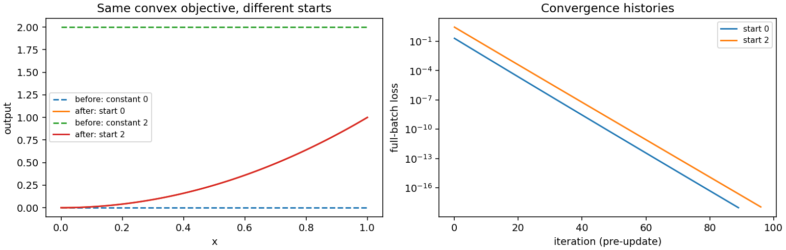
Fig. 32 A current-API before/after experiment with the same convex scalar response loss and two initial constants. Both reach the checked full-sample gradient tolerance. Unlike the historical research figures above, this figure is regenerated by the guide script and records its own termination evidence.

Run python examples/generate_guide_figures.py to reproduce this comparison. The generated JSON includes final objectives, iteration counts and statuses. The example uses a supervised-looking custom scalar loss only to provide an analytic reference for the optimizer; direct fit is the simpler operation for that particular quadratic regression task.

For a nonconvex application, repeat under several initial models and seeds, inspect feasibility across the domain, and compare independent evaluation objectives. No optimizer status certifies that a local stationary point is a global optimum or that linear scalarization covers unsupported nonconvex Pareto regions. Preserve the loss definition and units with the model archive so that later users can reproduce what was actually minimized.

A checklist for a new objective

First establish a baseline that can be evaluated without optimization. Predict from the initial model over a small independent grid, compute the row losses, and check that all decision vectors are feasible for the objective. If there is an analytic solution for a simplified case, test that case before increasing degree or adding a complicated simulator-derived cost. A complicated loss can produce plausible-looking curves even when objective columns or preference weights have been swapped.

Next check differentiation at an ordinary interior parameter point. The loss should depend on predicted values through finite PyTorch operations. A piecewise formula can be differentiable almost everywhere while having unhelpful gradients at a chosen constant start. Move the start or reformulate the smooth approximation deliberately, and record the choice. Increasing an iteration budget will not repair a detached graph or a gradient that is identically zero for an unintended reason.

Then separate algorithmic error from representation error. A converged low-degree model may still approximate the desired decision map poorly. Increase degree only after checking the same objective and independent points. Conversely, a flexible model with a large gradient may simply need a better numerical configuration before more controls are justified. Compare both final loss and convergence status rather than using either in isolation.

Finally retain enough evidence to reproduce the result: initial coefficients, space geometry, fixed controls, loss definition, penalties, point coordinates, seeds and complete method settings. The saved numerical model predicts outputs, but it does not serialize the Python callable defining the optimization task. A later user needs that callable and its objective units to interpret the reported final objective or continue an experiment reliably.

Preconditioner storage and repeated solves

With preconditioner="none" and no smoothness penalty, updates use elementwise arithmetic. No control-by-control matrix is constructed, including ridge-only runs, where the denominator is 1 + 2 * alpha * ridge with alpha the current decayed step size. Gram metrics and smoothness still require dense control matrices. Their LU factorization is reused when the matrix is constant: constant learning rates, or either decay schedule without penalties. A square-root learning-rate schedule with active regularization changes the matrix and recomputes its factorization each update. Fixed controls select the same free-control submatrix as the reference solve.

Run the public optimizer benchmark from a checkout with:

PYTHONPATH=. python examples/benchmark_minimize.py \
    --controls 16 64 256 --iterations 5 20 --repeats 3 \
    --output minimize-benchmark.json

Each size, budget and preconditioner runs in a fresh CPU process. JSON records Python/PyTorch/platform versions, float64 precision, threads, two output columns, elapsed optimizer time, pre-optimizer high-water RSS and total peak RSS. Imports and input construction are outside the timer but contribute to RSS; use multiple trials on the same machine to assess variation. Unit tests count allocations and factorizations and compare mathematical updates rather than asserting seconds. The legacy tests/benchmark.py suite also includes public minimize cases.

One macOS arm64/Python 3.13.12/PyTorch 2.10.0 CPU run with one thread compared the previous solves with these updates. At 16 controls and 20 updates, plain SGD took 0.033 s before and 0.036 s after, with peak RSS 222.0/223.1 MiB. At 64 controls it took 0.092/0.092 s and 223.4/222.9 MiB; Gram updates took 0.092/0.092 s and 226.7/223.8 MiB. These single trials illustrate the benchmark format; they do not establish a reliable speedup or a reduction in whole-process peak memory. The allocation and factorization counts establish the computational savings.

The benchmark separately profiles basis construction, outside its time/RSS measurement: fixed full batches currently construct local bases once per update plus the final evaluation. Reusing those blocks would require preserving the parameter-coordinate autograd graph across updates and handling minibatch row selection. That change is deferred; this optimization does not introduce a global dense basis or change differentiation through sample coordinates.