Elastic Net Model Selection
A canonical and highly practical application of this theory is hyperparameter optimization for the Elastic Net. In machine learning and statistics, selecting the correct regularization parameters is critical to balancing data fidelity, model sparsity, and numerical stability.
Traditional approaches rely on exhaustive grid searches or cross-validation over a discrete set of hyperparameter combinations \((\alpha, \lambda)\). This process is computationally expensive. By formulating the hyperparameter tuning as a multi-objective optimization problem over a regularization map [BS19], PyTorch-BSF allows for a continuous exploration of the model space, often reducing the computational cost by orders of magnitude (e.g., achieving speeds up to 2,000 times faster than exhaustive search for a 3-objective problem).
Unified Framework for Sparse Modeling
The Elastic Net example is part of a broader framework for generalized sparse modeling. Any optimization problem expressed as a convex combination of several strongly convex functions can be analyzed using this approach:
where \(f_m\) represent different aspects of the model, such as data fidelity (loss functions) or structural priors (regularization terms). By ensuring each \(f_m\) is strongly convex (e.g., by adding a small \(L_2\) penalty \(\frac{\epsilon}{2} \|\beta\|_2^2\)), the resulting solution map \(x^*(w)\) is guaranteed to be weakly simplicial [MHI21], allowing for high-quality approximation via Bézier simplices.
This unified framework extends far beyond the standard Elastic Net:
Generalized Linear Models (GLMs): The loss term can be any negative log-likelihood with a canonical link function (e.g., Logistic, Poisson, or Gamma regression).
Structural Regularization: Practitioners can incorporate structural priors like Group Lasso [YL06], Fused Lasso [TSR+05], or Smoothed Lasso to encode spatial or group relationships between features.
Transfer Learning and Covariate Shift: By using importance-weighted empirical risk as the loss function, the framework can handle scenarios where the training and test data distributions differ (covariate shift).
Robust Estimation: Replacing the standard squared error with robust loss functions like the Huber loss allows for model selection that is resilient to outliers.
Elastic Net Formulation
For the standard Elastic Net, the underlying multi-objective problem involves simultaneously minimizing three objectives over the model weights \(\beta \in \mathbb{R}^N\):
where \(n\) is the number of observations and \(\epsilon > 0\) is a small constant ensuring strong convexity. These correspond to the hyperparameter mapping \(w = (w_1, w_2, w_3)\) where:
By training the model on a sparse subset of weight vectors \(w\) and fitting a Bézier simplex, we obtain a continuous solution map \((x^*, f \circ x^*): \Delta^{M-1} \to G^*(f)\) that maps any weight \(w\) to the optimal weights \(\beta\) and the corresponding objective values.
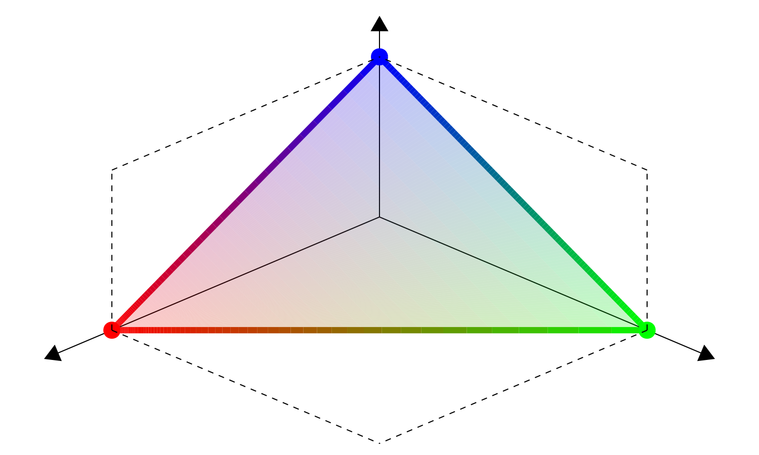
Fig. 8 Weight space \(\Delta^{2}\) |
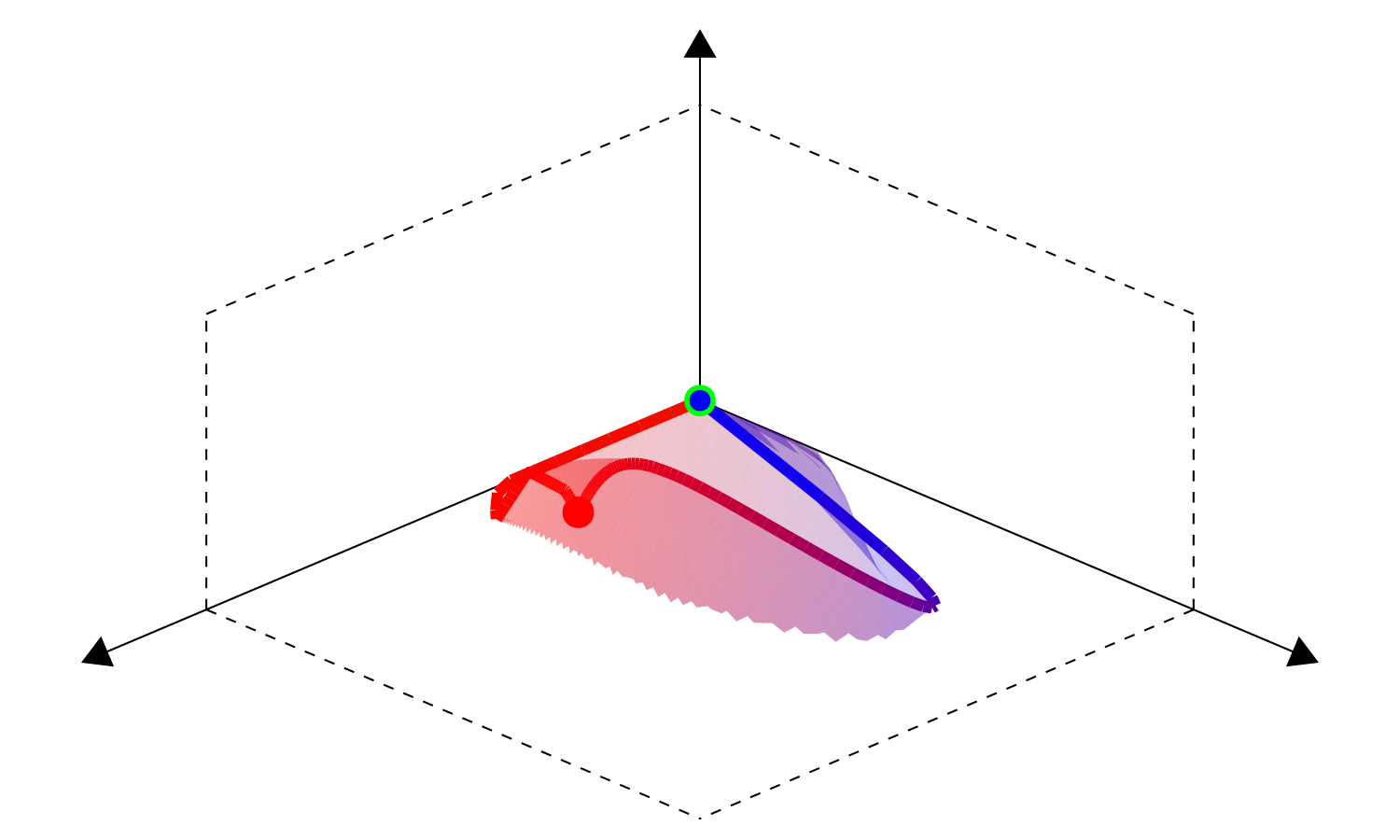
Fig. 9 Parameter space \(\Theta^*(f)\) |
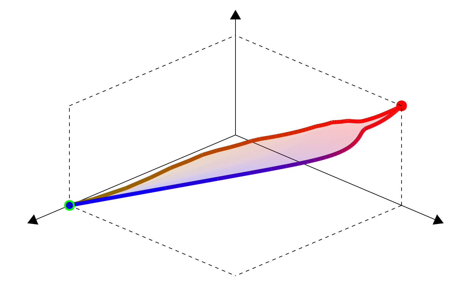
Fig. 10 Objective space \(f(\Theta^*(f))\) |
Model Selection on the Regularization Map
The resulting Bézier simplex provides a continuous surrogate of the performance surface, enabling users to apply various statistical model selection criteria analytically:
Minimum Cross-Validation Error (min profile rule): Locates the model \(w\) that minimizes the mean cross-validation error across folds, prioritizing predictive accuracy.
One Standard Error Rule (1se profile rule): Selects the most parsimonious (sparsest) model whose mean error is within one standard error of the minimum. This heuristic is widely used in tools like glmnet to gain stability and interpretability.
AICc Profile Rule: Balances goodness-of-fit and model complexity using the Akaike Information Criterion with Finite Sample Correction. This allows for selecting models with a theoretically grounded trade-off without the noise of fold-wise cross-validation variability.
Interactive Exploration and Insights
The Bézier simplex approximation of the regularization map provides more than just a tool for optimization. It offers a face structure that naturally reflects the combinations of subsets of loss and regularization terms. By observing the solutions on each face of the simplex, users can:
Obtain Insights: Gain a deep understanding of the trade-offs between different modeling assumptions, such as \(L_1\) vs \(L_2\) regularization.
Perform Exploratory Analysis: Test how sensitive the optimal model is to changes in hyperparameters without the trial-and-error of retraining.
Support Model Selection: Make better decisions a posteriori by seeing the entire landscape of potential models, rather than relying on a single fixed structure chosen a priori.
Empirical Evaluation
The effectiveness of PyTorch-BSF for Elastic Net is demonstrated using the Wine dataset from the UCI Machine Learning Repository. Experiments show that even with a limited number of training points (e.g., 51 points for a degree-6 simplex), the Bézier simplex accurately approximates the entire solution map, maintaining low Mean Squared Error (MSE) across the continuous hyperparameter space.
The following tables compare the results obtained through an exhaustive grid search (ground truth) and the Bézier simplex approximation. The high similarity between the performance surfaces confirms the fidelity of the surrogate model.
Fig. 11 Mean CV error |
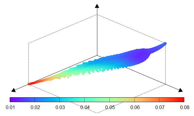
Fig. 12 Std dev of CV error |
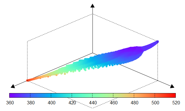
Fig. 13 AICc |
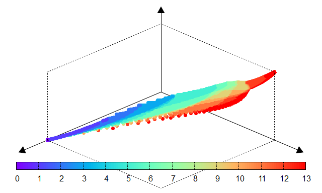
Fig. 14 Number of nonzero coefficients |

Fig. 15 Mean CV error |

Fig. 16 Std dev of CV error |

Fig. 17 AICc |

Fig. 18 Nonzero coefficients |