Elastic Net Grid Sampling

When fitting a Bézier simplex to the elastic-net regularization map you first need to choose a set of weight vectors on the standard 2-simplex \(\Delta^2\) at which to evaluate the model. The elastic_net_grid() function generates a purpose-built grid that respects the intrinsic geometry of the elastic-net hyperparameter space.

The Hyperparameter Space

The standard Elastic Net regression problem is formulated as:

\[\min_{\beta \in \mathbb{R}^N} \frac{1}{2n}\|y - X\beta\|_2^2 + \lambda \Bigl(\alpha \|\beta\|_1 + \frac{1-\alpha}{2}\|\beta\|_2^2\Bigr)\]

where \(\lambda \ge 0\) is the overall regularization strength and \(\alpha \in [0, 1]\) controls the L1/L2 mixing ratio (setting \(\alpha = 1\) recovers the Lasso; \(\alpha = 0\) gives Ridge regression).

To cast this into the multi-objective framework, we identify three objectives over \(\beta \in \mathbb{R}^N\):

\[\begin{split}f_{\text{data}}(\beta) &= \frac{1}{2n}\|y - X\beta\|_2^2 + \frac{\epsilon}{2}\|\beta\|_2^2 \\ f_{\text{sparse}}(\beta) &= \|\beta\|_1 + \frac{\epsilon}{2}\|\beta\|_2^2 \\ f_{\text{smooth}}(\beta) &= \frac{1 + \epsilon}{2}\|\beta\|_2^2\end{split}\]

where \(n\) is the number of observations and \(\epsilon > 0\) is a small constant. It appears as \(\frac{\epsilon}{2}\|\beta\|_2^2\) in \(f_{\text{data}}\) and \(f_{\text{sparse}}\) to make those terms strongly convex, and it is absorbed into \(f_{\text{smooth}}\) via the coefficient \(\frac{1+\epsilon}{2}\). This ensures all three objectives are strongly convex, which is required for the solution map to be weakly simplicial; see What is Bézier simplex fitting? for a detailed discussion.

Equivalently, elastic-net optimization can be written as a convex combination of the same three objectives:

\[\min_{\beta} \; w_1 \, f_{\text{data}}(\beta) + w_2 \, f_{\text{sparse}}(\beta) + w_3 \, f_{\text{smooth}}(\beta), \qquad (w_1, w_2, w_3) \in \Delta^2.\]

The conventional elastic-net parameters \(\lambda \ge 0\) (overall regularization strength) and \(\alpha \in [0, 1]\) (L1 mixing ratio) relate to the simplex weight vector by:

\[w_1 = \frac{1}{1+\lambda}, \qquad w_2 = \frac{\lambda\,\alpha}{1+\lambda}, \qquad w_3 = \frac{\lambda\,(1-\alpha)}{1+\lambda}.\]

With these weights the convex-combination objective equals the \(\epsilon\)-regularized elastic net objective divided by the positive constant \((1 + \lambda)\). Because this scale factor does not depend on \(\beta\), both formulations share the same minimizer.

The \((\lambda, \alpha)\) parameter space is a semi-infinite rectangle \([0,\infty) \times [0,1]\). When \(\lambda = 0\) the regularization terms vanish and the solution depends only on the data, regardless of \(\alpha\). Therefore the entire edge \(\{\lambda = 0\} \times [0, 1]\) maps to the single vertex \((w_1, w_2, w_3) = (1, 0, 0)\) of the simplex. Identifying this edge with a single point transforms the rectangle into a triangle – the 2-simplex \(\Delta^2\).

Conversely, as \(\lambda \to \infty\) the regularization overwhelms the data term and drives all model coefficients to zero, regardless of \(\alpha\). In the elastic net this limit is called the null model (all \(\beta_i = 0\)). All weight vectors on the opposite edge of the simplex \(\{(w_1, w_2, w_3) : w_1 = 0\}\) — the base edge connecting \((0, 1, 0)\) and \((0, 0, 1)\) — therefore correspond to the same solution. Since the Bézier simplex (and the underlying solution map) must assign a single output to each input weight, all of these base-edge weights are identified with a single null-model point \(P^*\) in the solution space. The elastic_net_grid() function still returns multiple distinct base-edge weights (\(w_1 = 0\) with varying \(w_2\), \(w_3\)), but they all evaluate to this same null-model solution. The resulting quotient space is a leaf/eye-shaped CW complex: two 0-cells (\(A\) and \(P^*\)), two 1-cells (the former edges \(AB\) and \(AC\), now connecting \(A\) to \(P^*\) as curves), and one 2-cell (the interior).

This identification gives the interior a leaf (foliation) structure: for each fixed value of \(w_1 \in (0, 1]\), the set of corresponding weight vectors \(\{(w_1, w_2, w_3) : w_2 + w_3 = 1 - w_1,\; w_2, w_3 \ge 0\}\) is a line segment (a leaf) parametrized by \(\alpha\). As \(w_1 \to 0\) (i.e. \(\lambda \to \infty\)), the images of these leaves under the solution map shrink to the single null-model point \(P^*\).

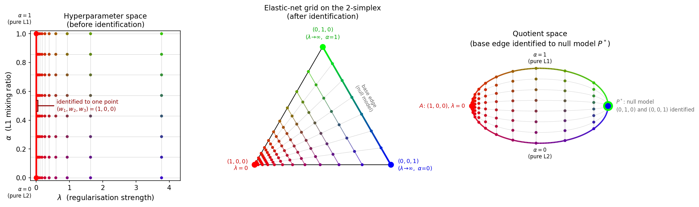
../_images/elastic_net_leaf_space.png — Fig. 10 All points are colored by \((w_1, w_2, w_3) \mapsto (R, G, B)\), so the same weight vector has the same color in every panel. **Left** – The \((\lambda, \alpha)\) hyperparameter space (x: regularization strength, y: L1 mixing ratio). The red line at \(\lambda = 0\) is the identified edge; all points on it share the color \((1, 0, 0)\) = red because \(w = (1, 0, 0)\) there. **Center** – The 2-simplex with vertices \((1,0,0)\) at the bottom-left (red), \((0,1,0)\) at the top (green), and \((0,0,1)\) at the bottom-right (blue). The gradient right edge (green→blue) is the null-model base edge to be identified. **Right** – The quotient space: vertex \(A\) = \((1,0,0)\) (red) at the left, and the null-model point \(P^*\) at the right shown as a large green dot \((0,1,0)\) behind a smaller blue dot \((0,0,1)\), reflecting that both endpoints of the base edge are identified to \(P^*\).

Grid Structure

A uniform grid in \((\lambda, \alpha)\) is sub-optimal because solutions change rapidly near \(\lambda = 0\) and slowly for large \(\lambda\). elastic_net_grid() therefore uses:

Log-scale spacing in the data-fidelity weight coordinate \(w_1\) – the reverse_logspace() routine generates n_lambdas - 1 values of \(w_1 \in [0, 1)\) that serve as \(w_1\)-levels for iso-\(w_1\) leaves, including \(w_1 = 0\) (which lies on the null-model base edge and corresponds to \(\lambda = \infty\)) and excluding the data-fidelity vertex at \(w_1 = 1\). The vertex at \(w_1 = 1\) (i.e. \(\lambda = 0\)) is appended separately. As \(w_1\) increases from 0 towards 1, these levels move from the base edge into the simplex interior towards the data-fidelity vertex. Since \(\lambda = (1 - w_1) / w_1\) is finite only for \(w_1 > 0\), all finite values of \(\lambda\) arise from \(0 < w_1 < 1\). The log spacing in \(w_1\) produces more \(w_1\) levels close to the data-fidelity vertex and therefore near \(\lambda = 0\). The steepness of this clustering is controlled by the base parameter: base=1 gives uniform spacing in \(w_1\), while larger values concentrate points further towards \(w_1 = 1\) (i.e. towards smaller \(\lambda\)).
Uniform spacing along \(\alpha\) – for each \(w_1\) level, the n_alphas values of \(\alpha\) are placed uniformly in \([0, 1]\) to span the corresponding iso-\(w_1\) leaf.

The n_vertex_copies parameter adds extra copies of each simplex vertex. This is useful when the grid is passed to k-fold cross-validation (see Automatic Degree Selection): set n_vertex_copies >= k for k-fold CV so that, when the fold-splitting procedure distributes rows approximately evenly, each fold will contain every vertex at least once. Using fewer copies than folds can inflate cross-validation variance.

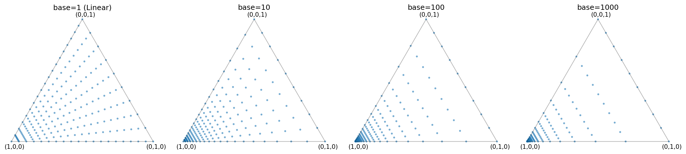
../_images/elastic_net_grid_comparison.png — Fig. 11 Grid points on the 2-simplex for different values of the `base` parameter (`n_lambdas=20`, `n_alphas=10`). Larger bases push more points towards the data-fidelity vertex \((1, 0, 0)\) (bottom-left corner in the figure), which is appropriate when you expect the optimal model to have small \(\lambda\).

Usage

As a Python Function

import numpy as np
from torch_bsf.model_selection.elastic_net_grid import elastic_net_grid

# Generate a grid with 102 lambda levels, 12 alpha levels, and 10 vertex
# copies (useful for 10-fold cross-validation).
grid = elastic_net_grid(
    n_lambdas=102,
    n_alphas=12,
    n_vertex_copies=10,
    base=10,
)
# grid.shape == (1240, 3)
# Each row is a weight vector (w1, w2, w3) on the 2-simplex.

np.savetxt("weights.csv", grid, delimiter=",", fmt="%.17e")

The returned array can be saved to a CSV file and then either (a) loaded back into an array or tensor and passed as the params argument to torch_bsf.fit(), or (b) passed as a file path to the --params CLI option, to train a Bézier simplex over the elastic-net regularization map.

As a Python Module (CLI)

Run the module directly to print the grid as a CSV file to stdout:

python -m torch_bsf.model_selection.elastic_net_grid \
    --n_lambdas=102 \
    --n_alphas=12 \
    --n_vertex_copies=10 \
    --base=10 \
    > weights.csv

All four parameters are optional and fall back to their defaults (n_lambdas=102, n_alphas=12, n_vertex_copies=1, base=10).

Via MLproject

The elastic_net_grid entry point in MLproject calls the same module and redirects the output to a CSV file named weight_{n_lambdas}_{n_alphas}_{n_vertex_copies}_{base}.csv:

mlflow run https://github.com/opthub-org/pytorch-bsf \
    -e elastic_net_grid \
    -P n_lambdas=102 \
    -P n_alphas=12 \
    -P n_vertex_copies=10 \
    -P base=10

After the run completes, the grid is saved in the current working directory as weight_102_12_10_10.csv. You can then pass it as the params argument to a subsequent training run:

mlflow run https://github.com/opthub-org/pytorch-bsf \
    -P params=weight_102_12_10_10.csv \
    -P values=values.csv \
    -P degree=6