Medical Imaging and Radiation Therapy

Optimizing diagnostic clarity and therapeutic safety simultaneously is paramount in medical fields, making multi-objective optimization frameworks indispensable.

For instance, Computed Tomography (CT) image reconstruction represents an ill-posed multi-objective inverse problem where doctors must minimize a data fidelity term (noise residual) against a regularization term safeguarding spatial continuity. Utilizing the L-Curve method [HOLeary93], this is routinely formulated mathematically as balancing:

\[\begin{split}f_1(x) &= \|Kx - y\|_2^2 \quad \text{(Fidelity)} \\ f_2(x) &= \|Lx\|_2^2 \quad \text{(Regularization)}\end{split}\]

Similarly, Intensity-Modulated Radiation Therapy (IMRT) requires treating patients via highly constrained inverse planning [BSK+07]. Planners must aggressively deliver prescriptive radiation doses to tumors while strictly repressing the doses affecting adjacent healthy Organs At Risk (OAR). The optimization minimizes heavily competing quadratic objectives:

\[s(f) = \sum_{v \in V} \xi_v (Hf - d_v^p)^T \tilde{\eta}_v (Hf - d_v^p) + \kappa (Mf)^T (Mf)\]

where the first component penalizes dose errors via beamlet fluence \(f\), and the second component applies spatial smoothing.

In both clinical environments, strong convexity critically anchors the computation. For CT reconstructions, the explicit \(L_2\) regularizations (via the parameter \(\lambda^2 \|Lx\|^2_2\)) stabilize singular projection matrices, resulting in a definitively positive-definite system matrix \(\nabla^2 f \succeq \lambda I\). Correspondingly, in IMRT, smoothing parameters (like \(\kappa\)) combined with dense beamlet mappings force the objective Hessian \(2(H^T \tilde{\eta} H + \kappa M^T M)\) to remain strictly positive definite.

In traditional practices, resolving the exact trade-offs requires hours of discrete algorithmic recalculations, delaying urgent therapies. However, by substituting the Pareto front mapping with a Bézier simplex, radiation oncologists and radiologists are granted an interactive, fully continuous digital slider. They can instantaneously sweep through the entire geometric space—trading off tumor destruction versus organ preservation precisely—in real-time without recalculating a single QP iteration.

Numerical Experiments

We illustrate Bézier simplex fitting on a small CT reconstruction problem, tracing the L-curve between data fidelity and spatial smoothness.

Problem Setup:

• Image: \(x \in \mathbb{R}^{256}\) (flattened 16×16 circular phantom)

• Forward operator: \(K \in \mathbb{R}^{128 \times 256}\) (simplified 2D Radon transform, 8 angles × 16 rays per angle)

• Finite-difference operator: \(L\) (2D anisotropic total variation, horizontal and vertical differences)

• Noisy measurement: \(y = Kx^* + \epsilon\) (\(\epsilon \sim \mathcal{N}(0, 0.05^2)\))

• Regularized objectives:

\[\begin{split}f_1(x) &= \|Kx - y\|^2 + 0.01\|x\|^2 \quad \text{(fidelity)} \\ f_2(x) &= \|Lx\|^2 + 0.01\|x\|^2 \quad \text{(smoothness)}\end{split}\]

Parametrization of the trade-off:

The weighted-sum solution \(x^*(w)\) depends only on the regularization parameter \(\lambda = w_2 / w_1\). Because \(K^\top K\) and \(L^\top L\) have nearly complementary spectra (smooth images are barely penalized by \(L\) but strongly seen by \(K\), and vice versa), \(x^*(w)\) has poles just outside the weight simplex: with uniformly spaced weights, almost all of the L-curve is squeezed into a tiny neighborhood of \(w = (1, 0)\), where no low-degree polynomial can follow it. As in the classical L-curve analysis, we therefore sweep \(\lambda\) on a logarithmic scale and fit the Bézier simplex on the parameter \((1 - t, t)\) of the 1-simplex:

\[\lambda(t) = 10^{-2 + 3t}, \qquad w(t) = \left(\frac{1}{1 + \lambda(t)}, \frac{\lambda(t)}{1 + \lambda(t)}\right), \qquad t \in [0, 1].\]

Experiment Procedure:

1. Sample 41 equally spaced parameters \(t \in [0, 1]\), i.e., \(\lambda\) from \(10^{-2}\) to \(10^{1}\).

2. For each \(t\), solve \(x^*(t) = \arg\min_x [w_1(t) f_1(x) + w_2(t) f_2(x)]\) using L-BFGS-B with the analytic gradient.

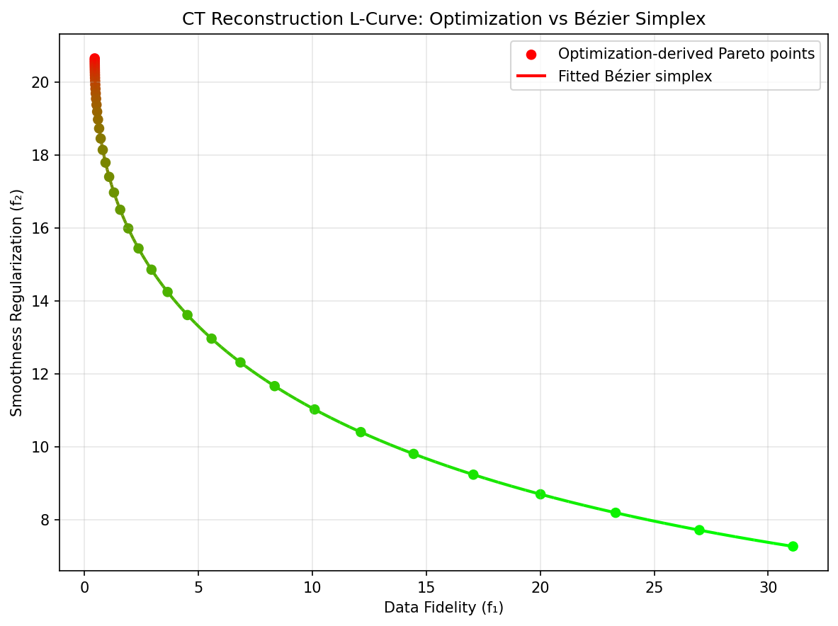
3. Collect the Pareto front points \((f_1(x^*(t)), f_2(x^*(t)))\) and the reconstructions \(x^*(t)\).

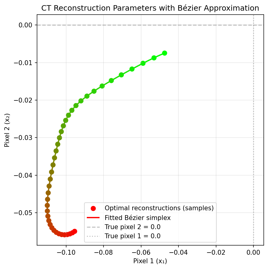
4. Fit degree-10 Bézier simplices to the Pareto front and to the Pareto set (the 256 pixels) by exact linear least squares (torch_bsf.fit()).

5. Evaluate the fitted Bézier curves on 20 held-out parameters between the training ones.

On the held-out parameters, the maximum error is about \(10^{-3}\) on the Pareto front (whose \(f_1\) ranges over \([0.4, 31]\)) and below \(10^{-4}\) per pixel on the Pareto set.

Pareto set (two background pixels).	Pareto front.

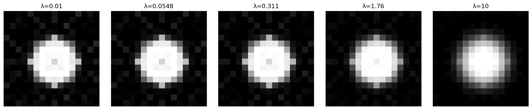
Fig. 39 Reconstructions predicted by the Bézier simplex fitted to the Pareto set, from weak (left) to strong (right) smoothing.

The complete example script is available at examples/generate_medical_imaging_pareto.py.