Multi-Objective Model Predictive Control

In industrial automation and robotics, Model Predictive Control (MPC) and Linear Quadratic Regulators (LQR) are foundational algorithms used to optimize future behavior in real-time. Operating chemical plant processes, for instance, requires rigorously balancing product quality tracking (setpoint proximity) against the suppression of abrupt heater and valve modifications (machinery wear).

Similarly, omnidirectional mobile robots traversing complex environments (e.g., hospitals or warehouses) must optimize trajectory tracking while minimizing energy consumption and avoiding collisions. However, they face significant physical constraints like nonlinear friction modes. Over a predictive horizon \(H\), these systems evaluate competing objectives to find the strictly optimal control sequence \(U\):

\[\begin{split}f_{track}(U) &= \sum_{k=1}^H \|y_k - r_k\|_Q^2 \\ f_{smooth}(U) &= \sum_{k=0}^{H-1} \|\Delta u_k\|_R^2 \\ f_{energy}(U) &= \sum_{k=0}^{H-1} \|u_k\|_S^2\end{split}\]

where \(y_k\) denotes system states/outputs, \(r_k\) the target setpoints, \(u_k\) the operational inputs, and \(\Delta u_k\) the input change rates.

Crucially, as long as the weighting matrices (e.g., \(R\)) acting on the independent control inputs are uniformly positive definite (\(R \succ 0\)), the resulting multi-objective performance stage cost is strongly convex with respect to the continuous input decisions \(U\). Even in complex scenarios where discrete mode switching (like robot friction statuses) transforms the formulation into a Mixed-Integer Quadratic Program (MIQP), the continuous sub-component remains undeniably strongly convex, stabilizing bounded-node optimization searches.

In practice, resolving these multi-objective QP or MIQP problems during an active millisecond control loop requires prohibitive amounts of computational power. Since the strong convexity naturally spans a continuous simplicial Pareto front, controllers equipped with a Bézier simplex representation can bypass the online QP solver entirely. The polynomial evaluation provides an analytic, instantaneous multi-objective control response, enabling ultra-fast, high-frequency continuous re-optimization in highly unstable physical environments.

Numerical Experiments

An MPC controller solves the same problem again at every sampling instant, each time from a different measured state. The optimal inputs therefore depend not only on the objective weights \(w\) but also on the initial state \(x_0\). Their joint parameter space is the product of the weight simplex and an interval, i.e., the square \(\Delta^1 \times \Delta^1\), which is a simploid rather than a simplex (see Simploidal Sets). We therefore fit a Bézier simploid of type \((1, 1)\) that represents, in one polynomial, the Pareto sets and fronts for all initial states — an explicit multi-objective MPC law.

Problem Setup:

• Stable 1D system: \(x(k+1) = 0.5\,x(k) + u_k\), target \(r = 1\), horizon \(H = 5\)

• Initial state: \(x(0) = x_0 \in [-1, 1]\)

• Control sequence: \(U = [u_0, u_1, u_2, u_3, u_4] \in \mathbb{R}^5\)

• Competing objectives:

\[\begin{split}f_1(U; x_0) &= \sum_{k=0}^{4} (x(k+1) - r)^2 \quad \text{(tracking error)} \\ f_2(U) &= \sum_{k=0}^{4} u_k^2 \quad \text{(control effort)}\end{split}\]

• Parameter of the simploid: \((w_1, w_2, v_1, v_2) \in \Delta^1 \times \Delta^1\) with \(x_0 = -v_1 + v_2\)

Both objectives are strongly convex in \(U\) with comparable curvature, so \(U^*(w, x_0)\) is a smooth rational function of \(w\). For a fixed \(w\), it is affine in \(x_0\), and the objective values are quadratic in \(x_0\).

Experiment Procedure:

1. Sample an \(11 \times 5\) grid on the square: 11 weight vectors from \(w = (1,0)\) to \((0,1)\) and 5 initial states from \(x_0 = -1\) to \(1\).

2. For each \((w, x_0)\), solve \(U^*(w, x_0) = \arg\min_U [w_1 f_1(U; x_0) + w_2 f_2(U)]\) using L-BFGS-B.

3. Collect the Pareto front points \((f_1, f_2)\) and the Pareto set points \(U^*\).

4. Fit Bézier simploids of type \((1, 1)\) with torch_bsf.fit(): degree \((6, 2)\) for the Pareto front and \((6, 1)\) for the Pareto set.

5. Evaluate the fitted simploids on a \(41 \times 21\) test grid.

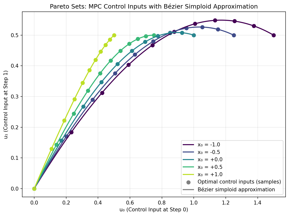
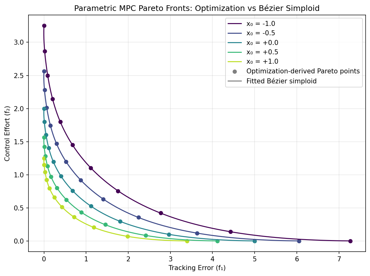
On the test grid, the maximum error is about \(0.01\) on the Pareto front (0.2% of the range of \(f_1\)) and below \(10^{-3}\) on the Pareto set. The figures show the curves of the fitted simploids for the five sampled initial states.

Pareto sets.	Pareto fronts.

The complete example script is available at examples/generate_mpc_pareto.py.