What is Bézier simplex fitting?

You are probably familiar with Bézier curves (1-D) and Bézier triangles (2-D) from computer graphics and CAD software. A Bézier simplex is their natural generalization to any number of dimensions: the same elegant polynomial construction, extended to an \((M-1)\)-dimensional surface defined over a standard simplex.

Just as a Bézier curve smoothly interpolates or approximates a 1-D point cloud using a small set of control points, a Bézier simplex can approximate a high-dimensional point cloud with excellent flexibility and mathematical guarantees.

This page introduces the formal definition of Bézier simplices, the least-squares fitting algorithm used by PyTorch-BSF, and motivating real-world applications.

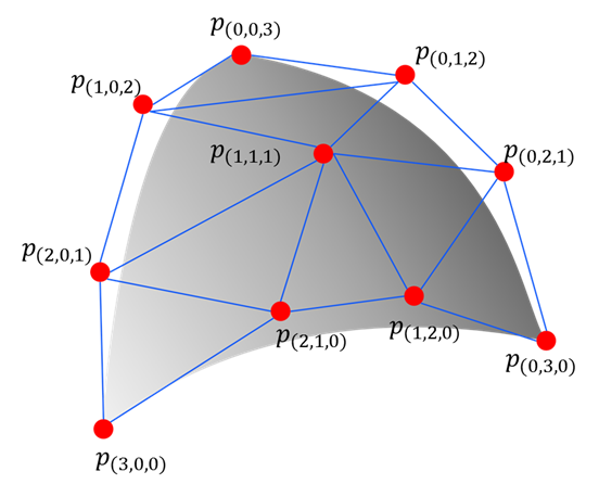
Bezier simplex

Let \(D, M, N\) be nonnegative integers, \(\mathbb N\) the set of nonnegative integers (including zero!), and \(\mathbb R^N\) the \(N\)-dimensional Euclidean space. We define the index set by

\[\mathbb N_D^M = \left\{\mathbf d=(d_1,\ldots,d_M)\in\mathbb N^M\ \Bigg|\ \sum_{m=1}^M d_m=D\right\},\]

and the simplex by

\[\Delta^{M-1} = \left\{\mathbf t=(t_1,\ldots,t_M)\in[0,1]^M\ \Bigg|\ \sum_{m=1}^M t_m=1\right\}.\]

An \((M-1)\)-dimensional Bezier simplex of degree \(D\) in \(\mathbb R^N\) is a polynomial map \(\mathbf b: \Delta^{M-1}\to\mathbb R^N\) defined by

\[\mathbf b(\mathbf t\mid\mathbf p) = \sum_{\mathbf d\in\mathbb N_D^M} \binom{D}{\mathbf d} \mathbf t^{\mathbf d} \mathbf p_{\mathbf d},\]

where \(\mathbf t^{\mathbf d} = t_1^{d_1} t_2^{d_2}\cdots t_M^{d_M}\), \(\binom{D}{\mathbf d}=D! / (d_1!d_2!\cdots d_M!)\), and \(\mathbf p_{\mathbf d}\in\mathbb R^N\ (\mathbf d\in\mathbb N_D^M)\) are parameters called the control points.

Fitting a Bezier simplex to a dataset

Assume we have a finite dataset \(B\subset\Delta^{M-1}\times\mathbb R^N\) and want to fit a Bezier simplex to the dataset. What we are trying can be formulated as a problem of finding the best vector of control points \(\mathbf p=(\mathbf p_{\mathbf d})_{\mathbf d\in\mathbb N_D^M}\) that minimizes the least square error between the Bezier simplex and the dataset:

\[\arg\min_{\mathbf p} \sum_{(\mathbf t,\mathbf x)\in B}\|\mathbf b(\mathbf t\mid\mathbf p)-\mathbf x\|^2.\]

PyTorch-BSF provides an algorithm for solving this optimization problem with the L-BFGS algorithm.

Why does Bézier simplex fitting matter?

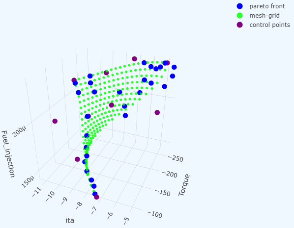
In multi-objective optimization the Pareto front — the set of all trade-off-optimal solutions — is rarely a single point; it is a surface. For a broad class of problems (see weakly simplicial problems below), that surface is well-approximated by a Bézier simplex.

This has a powerful practical consequence: instead of solving the optimization problem exhaustively for every possible weight vector, you can solve it for a small number of carefully chosen weights, fit a Bézier simplex to those solutions, and then read off the entire Pareto front by evaluating the fitted surface. A canonical application is hyperparameter search for the elastic net, where the two regularization coefficients \(\lambda\) and \(\alpha\) span exactly such a simplex.

Approximation theorem

Any continuous map from a simplex to a Euclidean space can be approximated by a Bezier simplex. More precisely, the following theorem holds. See [1] for technical details.

Weakly simplicial problems

Such a map \(\Phi\) arises in, e.g., multiobjective optimization. There exists a continuous map from a simplex to the Pareto set and Pareto front such that the map sends a subsimplex to the Pareto set/front of a subproblem. See [3].

Application 1: Elastic net

The elastic net objective combines L1 and L2 regularization with two coefficients, \(\lambda\) (overall strength) and \(\alpha\) (L1/L2 balance). Together they define a point on a 2-simplex, making the elastic net a natural fit for Bézier simplex methods.

Rather than running a grid search over all \((\lambda, \alpha)\) combinations, you can solve the elastic net for a small set of simplex-structured weight vectors, fit a Bézier simplex to the resulting (solution, loss) pairs, and evaluate the surface densely at negligible cost. See [3] for the theoretical guarantees.

Strongly convex problems

All unconstrained strongly convex problems are weakly simplicial [3].

Weighted-sum scalarization and solution map

The weighted-sum scalarization \(x^*: \Delta^{M-1}\to\mathbb R^N\) defined by

\[x^*(w)=\arg\min_x \sum_{m=1}^M w_m f_m(x).\]

We define the solution map \((x^*,f\circ x^*):\Delta^{M-1}\to G^*(f)\) by

\[(x^*,f\circ x^*)(w)=(x^*(w),f(x^*(x))).\]

The solution map is continuous and surjective. See [3] for technical details.

Application 2: Deep neural networks

Training a GAN involves balancing multiple competing losses. For consistency-regularized GANs (bCR / zCR), the generator and discriminator objectives combine several loss terms whose relative weights form a simplex structure. Fitting a Bézier simplex to solutions sampled across this simplex reveals the full trade-off surface without re-training from scratch for each configuration.

Concretely, the discriminator and generator losses are defined as

\[ \begin{align}\begin{aligned}L_D^\mathrm{bCR}&=L_D+\lambda_\mathrm{real}L_\mathrm{real}+\lambda_\mathrm{fake}L_\mathrm{fake},\\L_D&=D(G(z))-D(x),\\L_\mathrm{real}&=\|D(x)-D(T(x))\|^2,\\L_\mathrm{fake}&=\|D(G(z))-D(T(G(z)))\|^2,\\L_D^\mathrm{zCR}&=L_D+\lambda_\mathrm{dis}L_\mathrm{dis},\\L_G^\mathrm{zCR}&=L_G+\lambda_\mathrm{gen}L_\mathrm{gen},\\L_G&=-D(G(z)),\\L_\mathrm{dis}&=\|D(G(z))-D(G(T(z)))\|^2,\\L_\mathrm{gen}&=\|G(z)-G(T(z))\|^2.\end{aligned}\end{align} \]

Statistical test for weakly simpliciality

When the problem class is not known in advance, it is not clear whether the Pareto set admits a simplex structure. A data-driven statistical test [4] can determine whether this assumption is warranted before committing to a Bézier simplex model. See [4] for the methodology and test statistics.

References

1. Kobayashi, K., Hamada, N., Sannai, A., Tanaka, A., Bannai, K., & Sugiyama, M. (2019). Bézier Simplex Fitting: Describing Pareto Fronts of Simplicial Problems with Small Samples in Multi-Objective Optimization. Proceedings of the AAAI Conference on Artificial Intelligence, 33(01), 2304-2313. https://doi.org/10.1609/aaai.v33i01.33012304

2. Tanaka, A., Sannai, A., Kobayashi, K., & Hamada, N. (2020). Asymptotic Risk of Bézier Simplex Fitting. Proceedings of the AAAI Conference on Artificial Intelligence, 34(03), 2416-2424. https://doi.org/10.1609/aaai.v34i03.5622

3. Mizota, Y., Hamada, N., & Ichiki, S. (2021). All unconstrained strongly convex problems are weakly simplicial. arXiv:2106.12704 [math.OC]. https://arxiv.org/abs/2106.12704

4. Hamada, N. & Goto, K. (2018). Data-Driven Analysis of Pareto Set Topology. Proceedings of the Genetic and Evolutionary Computation Conference, 657-664. https://doi.org/10.1145/3205455.3205613