Quickstart

Create a polynomial space, observations, and an explicit fit result:

import torch
from torch_bsf import BezierSpace, Samples, fit

space = BezierSpace.simplex(dimension=1, degree=2)
t = torch.tensor([[1., 0.], [.5, .5], [0., 1.]])
result = fit(space, Samples(t, [[0.], [1.], [4.]]))
result.require_success()
predictions = result.model(t)
print(result.metrics)

BezierSpace contains immutable geometry and coefficient ordering. Dimensions, polynomial degrees and control multi-indices must be Python or NumPy integers. Floats (even 2.0), booleans and numeric strings raise ValueError rather than being silently converted. A simplex may have dimension zero; simploid factor dimensions are positive. Single-cell spaces allow degree zero, while spaces compiled from a shared topology require positive degrees. BezierModel contains the learned coefficients and is a PyTorch module. fit always returns FitResult; predict through result.model. No Lightning, MLflow or Conda installation is required for this example.

The command line uses the same operations:

python -m torch_bsf fit --params params.csv --values values.csv --degree 2 --save model.bsf
python -m torch_bsf predict --model model.bsf --params params.csv --save predictions.csv
python -m torch_bsf cross-validate --params params.csv --values values.csv --degree 2 --folds 3
python -m torch_bsf select-degree --params params.csv --values values.csv --degree 1 --degrees 1 2 3 --folds 3

Outputs include metrics and numerical status. An unsuccessful numerical solve returns a nonzero exit code. Tracking is opt-in with fit --track. Run bash examples/quickstart/run.sh for a complete local example. See Command-line reference for all five subcommands, CSV layouts, a self-contained minimize example, and exit codes and model-saving rules.

Persistence uses one versioned, non-pickled format:

from torch_bsf.io import save_model, load_model
save_model("model.bsf", result.model)
restored = load_model("model.bsf")

The extension does not choose a different format. CSV export is a separate export_control_points operation and does not preserve geometry.

Verified Python workflow

The following example exercises fixed constraints, cross-validation, objective minimization, and persistence using the same space and model types.

import tempfile
from pathlib import Path
import torch
from torch_bsf import (
    BezierSpace, FixedControls, Samples, fit, minimize, PreconditionedSGD,
)
from torch_bsf.sampling import grid
from torch_bsf.model_selection import KFold, cross_validate
from torch_bsf.io import save_model, load_model

space = BezierSpace.simplex(1, degree=2)
points = grid(space, resolution=12)
observations = Samples(points, points.parameters[:, :1] ** 2)
fixed = FixedControls({space.control_index((2, 0)): [1.]})
result = fit(space, observations, fixed=fixed)
assert result.success and result.metrics["data_mse"] < 1e-24
validation = cross_validate(space, observations, cv=KFold(3, seed=7))
assert validation.success and validation.metrics["pooled_mse"] < 1e-24
optimized = minimize(
    result.model, lambda y, p: (y[:, 0] - p.parameters[:, 0] ** 2).square(),
    points=points, method=PreconditionedSGD(gradient_tolerance=1e-8),
)
assert optimized.success
with tempfile.TemporaryDirectory() as directory:
    destination = Path(directory) / "model.bsf"
    save_model(destination, optimized.model)
    restored = load_model(destination)
    assert torch.equal(restored(points), optimized.model(points))

To predict a saved multi-cell model, pass --cell-ids cells.csv with one integer cell ID per row and pad parameter rows to the saved space width.

A one-column parameter CSV denotes a constant domain when dimensions are inferred. The column is a dummy input and is ignored for both fitting and prediction of zero-dimensional models.

Prepare your own observations

Use regression when you know response values at parameter locations and want a continuous surrogate between them. For a segment, write each normalized setting x as two coordinates [1-x, x]. The two input columns sum to one; they are not independent predictors. On a triangle, use three nonnegative coordinates summing to one. Product domains concatenate one such block per factor; see Single and assembled domains before preparing product data.

Parameter and value files must contain the same number of rows in corresponding order. Each value row contains one or more output columns. An input location without a measured response is a prediction request, not a training row. The following files fit the quadratic example at the top of this page:

cat > params.csv <<'EOF'
1.0,0.0
0.5,0.5
0.0,1.0
EOF
cat > values.csv <<'EOF'
0.0
1.0
4.0
EOF
python -m torch_bsf fit --params params.csv --values values.csv --degree 2 --save model.bsf
python -m torch_bsf predict --model model.bsf --params params.csv --save predictions.csv

These commands explicitly choose a model destination and a prediction destination. The saved model includes its polynomial space, so prediction needs no degree argument. Predict at a different file of valid parameter rows to evaluate interpolation. Keep predicted values separate from original observations; appending predictions as if they were new measurements does not add information.

Read results before choosing a more complicated model

result.metrics["data_mse"] describes weighted squared error averaged over output columns. objective additionally includes any ridge and smoothness penalties. Check numerical success first, then evaluate prediction quality. Even an exact training interpolation can behave poorly between noisy or sparse observations. A successful solve can also have unidentified coefficient directions; inspect diagnostics if data are scarce relative to controls.

Start with a low degree and no penalties. Increase degree only when held-out errors and plotted residuals support additional variation. If noise causes oscillation, compare lower degree, ridge or smoothness on the same folds. If an endpoint is known exactly, use fixed controls rather than a very large observation weight. The corresponding tutorials explain which settings change the polynomial space and which only choose coefficients within it.

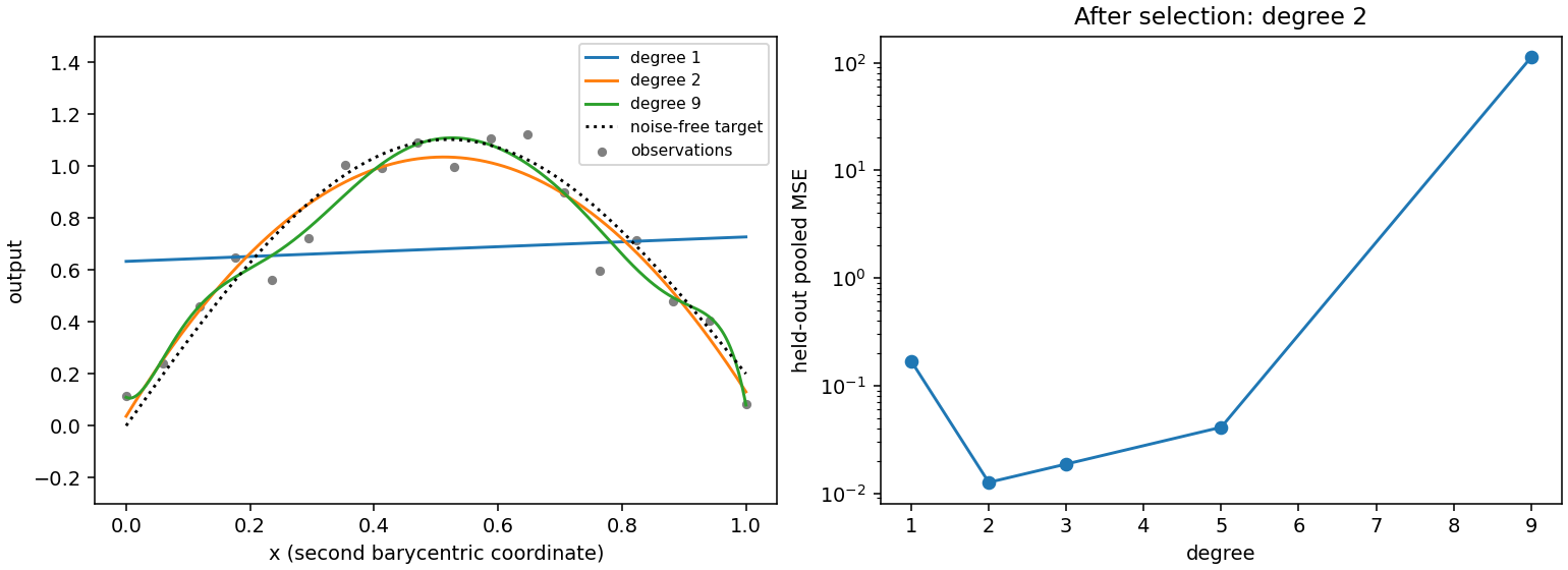
Fig. 1 A separate noisy-response example shows why training a higher-degree curve is not automatically an improvement. Choose with held-out error, then explicitly refit. See Cross-validation and degree search for the exact data, seed, candidate list and executable search.

Next steps and reproducibility

Use Visualization to overlay observations and fitted images, Output scaling when output units differ, and Sampling and grids to choose additional evaluation or measurement points. For an expensive experiment, Explicit ensembles and active learning shows how to query new true responses, append them and refit. For a cost defined by objectives rather than measured targets, use Objective minimization.

The CLI exposes operation-specific help, for example python -m torch_bsf fit --help. Tracking is explicit and requires the MLflow extra. Docker users can run the same subcommands inside the repository image with their working directory mounted. The repository’s MLproject describes MLflow project entry points, while the core Python examples require neither that service nor a Trainer.

To reproduce the current tutorial figures in a checkout, install the plot extra and run python examples/generate_guide_figures.py. The script records local seeds, settings and measured errors alongside its images. Save the raw observations, chosen space, validation settings and preprocessing statistics with each real experiment; the model archive preserves the predictor but does not automatically preserve every decision that led to it.